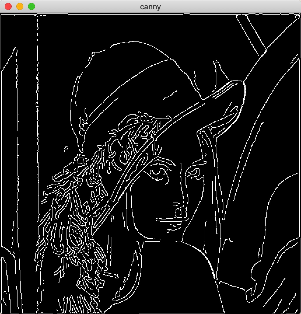
Canny边缘检测算法(基于OpenCV的Java实现) 绪论 最近在学习ORB的过程中又仔细学习了Canny,故写下此篇笔记,以作总结。
Canny边缘检测算法的发展历史 Canny边缘检测于1986年由JOHN CANNY首次在论文《A Computational Approach to Edge Detection》中提出,就此拉开了Canny边缘检测算法的序幕。
Canny边缘检测是从不同视觉对象中提取有用的结构信息并大大减少要处理的数据量的一种技术,目前已广泛应用于各种计算机视觉系统。Canny发现,在不同视觉系统上对边缘检测的要求较为类似,因此,可以实现一种具有广泛应用意义的边缘检测技术。边缘检测的一般标准包括:
以低的错误率检测边缘,也即意味着需要尽可能准确的捕获图像中尽可能多的边缘。
检测到的边缘应精确定位在真实边缘的中心。
图像中给定的边缘应只被标记一次,并且在可能的情况下,图像的噪声不应产生假的边缘。
为了满足这些要求,Canny使用了变分法。Canny检测器中的最优函数使用四个指数项的和来描述,它可以由高斯函数的一阶导数来近似。
在目前常用的边缘检测方法中,Canny边缘检测算法是具有严格定义的,可以提供良好可靠检测的方法之一。由于它具有满足边缘检测的三个标准和实现过程简单的优势,成为边缘检测最流行的算法之一。
Canny边缘检测算法的处理流程 Canny边缘检测算法可以分为以下5个步骤:
使用高斯滤波器,以平滑图像,滤除噪声。
计算图像中每个像素点的梯度强度和方向。
应用非极大值(Non-Maximum Suppression)抑制,以消除边缘检测带来的杂散响应。
应用双阈值(Double-Threshold)检测来确定真实的和潜在的边缘。
通过抑制孤立的弱边缘最终完成边缘检测。
下面详细介绍每一步的实现思路。
用高斯滤波器平滑图像 高斯滤波是一种线性平滑滤波,适用于消除高斯噪声,特别是对抑制或消除服从正态分布的噪声非常有效。滤波可以消除或降低图像中噪声的影响,使用高斯滤波器主要是基于在滤波降噪的同时也可以最大限度保留边缘信息的考虑。
高斯滤波实现步骤:
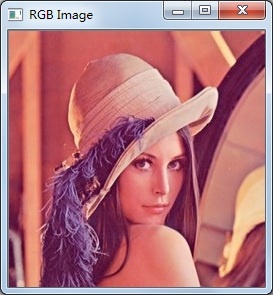
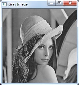
彩色RGB图像转换为灰度图像 边缘检测是基于对图像灰度差异运算实现的,所以如果输入的是RGB彩色图像,需要先进行灰度图的转换。
注意一般情况下图像处理中彩色图像各分量的排列顺序是B、G、R。
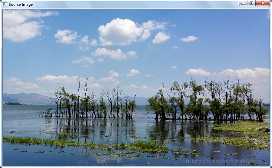
RGB原图像:
转换后的灰度图:
Java代码调用系统库实现:
1
2
3
4
5
6
public static Mat RGB2Gray (Mat image) Mat gray = new Mat(); Imgproc.cvtColor(image, gray, Imgproc.COLOR_BGR2GRAY); return gray; }
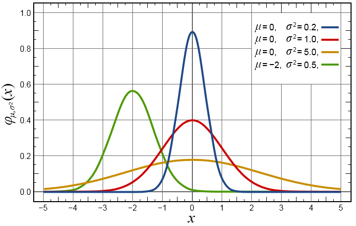
一维,二维高斯函数及分布 一维高斯函数表述为:
对应图形:
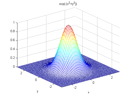
二维高斯函数表述为:
对应图形:
一些重要特性说明:
一维二维高斯函数中$μ$是服从正态分布的随机变量的均值,称为期望或均值影响正态分布的位置,实际的图像处理应用中一般取$μ=0;~σ$是标准差,$σ^2$是随机变量的方差,$σ$定义了正态分布数据的离散程度,$σ$越大,数据分布越分散,σ越小,数据分布越集中。
在图形或滤波效果上表现为:$σ$越大,曲线越扁平,高斯滤波器的频带就越宽,平滑程度就越好,$σ$越小,曲线越瘦高,高斯滤波的频带就越窄,平滑程度也越弱;
二维高斯函数具有旋转对称性,即滤波器在各个方向上的平滑程度是相同的.一般来说,一幅图像的边缘方向是事先不知道的,因此,在滤波前是无法确定一个方向上比另一方向上需要更多的平滑.旋转对称性意味着高斯平滑滤波器在后续边缘检测中不会偏向任一方向;
高斯函数是单值函数。这表明,高斯滤波器用像素邻域的加权均值来代替该点的像素值,而每一邻域像素点权值是随该点与中心点的距离单调增减的。这一性质是很重要的,因为边缘是一种图像局部特征,如果平滑运算对离算子中心很远的像素点仍然有很大作用,则平滑运算会使图像失真;
相同条件下,高斯卷积核的尺寸越大,图像的平滑效果越好,表现为图像越模糊,同时图像细节丢失的越多;尺寸越小,平滑效果越弱,图像细节丢失越少;
以下对比一下不同大小标准差$σ$(Sigma)对图像平滑的影响:
原图:
卷积核尺寸5*5,σ=0.1:
卷积核尺寸5*5,σ=1:
对比可以看到,Sigma(σ)越大,平滑效果越明显。
生成高斯滤波卷积核 滤波的主要目的是降噪,一般的图像处理算法都需要先进行降噪。而高斯滤波主要使图像变得平滑(模糊),同时也有可能增大了边缘的宽度。
高斯函数是一个类似与正态分布的中间大两边小的函数。
对于一个位置(m,n)的像素点,其灰度值(这里只考虑二值图)为f(m,n)。
那么经过高斯滤波后的灰度值将变为:
其中,
是二元高斯函数。
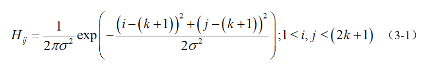
为了尽可能减少噪声对边缘检测结果的影响,所以必须滤除噪声以防止由噪声引起的错误检测。为了平滑图像,使用高斯滤波器与图像进行卷积,该步骤将平滑图像,以减少边缘检测器上明显的噪声影响。大小为(2k+1)x(2k+1)的高斯滤波器核的生成方程式由下式给出:
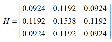
下面是一个sigma = 1.4,尺寸为3x3的高斯卷积核的例子(需要注意归一化):
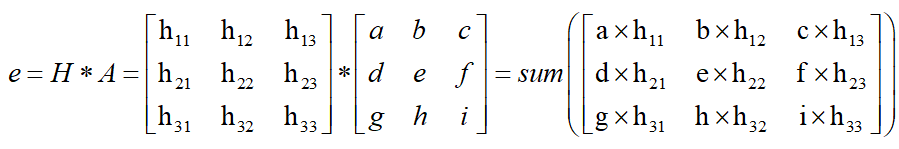
若图像中一个3x3的窗口为A,要滤波的像素点为e,则经过高斯滤波之后,像素点e的亮度值为:
其中*为卷积符号,sum表示矩阵中所有元素相加求和。
重要的是需要理解,高斯卷积核大小的选择将影响Canny检测器的性能。尺寸越大,检测器对噪声的敏感度越低,但是边缘检测的定位误差也将略有增加。一般5x5是一个比较不错的trade off。
1
2
3
4
5
6
7
8
9
10
11
12
13
14
15
16
public static double [][] getGaussianArray(int size, double sigma) { double [][] array = new double [size][size]; double center_i, center_j; if (size % 2 == 1 ) { center_i = (double ) (size / 2 ); center_j = (double ) (size / 2 ); } else { center_i = (double ) (size / 2 ) - 0.5 ; center_j = (double ) (size / 2 ) - 0.5 ; } double sum = 0.0 ; for (int i = 0 ; i < size; i ++) for (int j = 0 ; j < size; j ++) { array[i][j] = Math.exp((-1.0 ) * ((i - center_i) * (i - center_i) + (j - center_j) * (j - center_j)) / 2.0 / sigma / sigma); sum += array[i][j]; } for (int i = 0 ; i < size; i ++) for (int j = 0 ; j < size; j++) array[i][j] /= sum; return array; }
Sigma为1时,求得的3*3大小的高斯卷积核参数为:
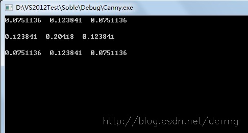
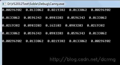
Sigma为1,5*5大小的高斯卷积核参数为:
在计算出高斯滤波卷积核之后就是用这个卷积核来扫过整张图像,对每个像素点进行加权平均。
单色高斯滤波与彩色高斯滤波 加入了多线程的优化,代码实现:
1
2
3
4
5
6
7
8
9
10
11
12
13
14
15
16
17
18
19
20
21
22
23
24
25
26
27
28
29
30
31
32
33
34
35
36
37
38
39
40
41
42
43
44
45
46
47
48
49
50
51
52
53
public static Mat greyGaussianFilter (Mat src, double [][] array, int size) throws InterruptedException Mat temp = src.clone(); final CountDownLatch latch = new CountDownLatch(src.rows()); for (int i = 0 ; i < src.rows(); i ++) { int finalI = i; new Thread(() -> { for (int j = 0 ; j < src.cols(); j ++) if (finalI > (size / 2 ) - 1 && j > (size / 2 ) - 1 && finalI < src.rows() - (size / 2 ) && j < src.cols() - (size / 2 )) { double sum = 0.0 ; for (int k = 0 ; k < size; k++) for (int l = 0 ; l < size; l++) sum += src.get(finalI - k + size / 2 , j - l + size / 2 )[0 ] * array[k][l]; temp.put(finalI, j, sum); } latch.countDown(); }).start(); } latch.await(); return temp; } public static Mat colorGaussianFilter (Mat src, int size, double sigma) throws InterruptedException Mat ret = new Mat(); List<Mat> channels = new ArrayList<>(); List<Mat> new_channels = new ArrayList<>(); Map<Integer, Mat> temp_channels = new TreeMap<>(); Core.split(src, channels); double [][] array = SmartGaussian.getGaussianArray(size, sigma); final CountDownLatch latch = new CountDownLatch(channels.size()); channels.forEach(mat -> { new Thread(() -> { Mat tmp = new Mat(); try { tmp = SmartGaussian.greyGaussianFilter(mat, array, size); } catch (InterruptedException e) { e.printStackTrace(); } temp_channels.put(channels.indexOf(mat), tmp); latch.countDown(); }).start(); }); latch.await(); for (int i = 0 ; i < channels.size(); i ++) new_channels.add(temp_channels.get(i)); Core.merge(new_channels, ret); return ret; }
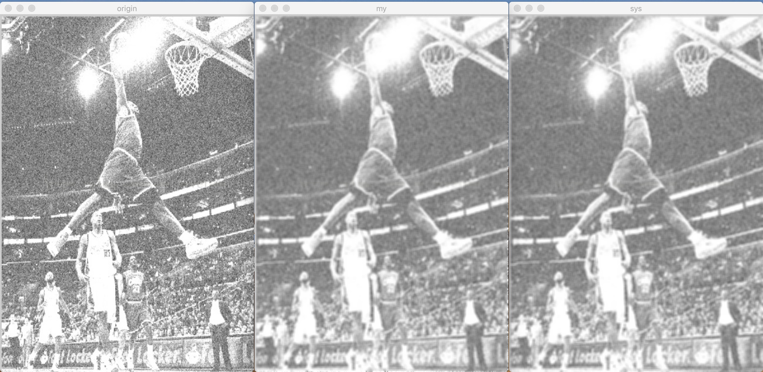
效果图:(左图为原图,中间为上面的实现,右边是OpenCV实现)
用Sobel等梯度算子计算梯度幅值和方向 梯度 梯度的本意是一个向量(矢量),表示某一函数在该点处的方向导数沿着该方向取得最大值,即函数在该点处沿着该方向(此梯度的方向)变化最快,变化率最大(为该梯度的模)。
设二元函数:
在平面区域D上具有一阶连续偏导数,则对于每一个点$P(x,y)$都可定出一个向量:
该函数就称为函数$z=f(x,y)$在点$P(x,y)$的梯度,记作$\text{grad}~f(x,y)$或$\nabla f(x,y)$,即有:
其中$\nabla=\displaystyle\frac{\partial}{\partial x}\vec i+\displaystyle\frac{\partial}{\partial y}\vec j$称为(二维的)向量微分算子 或Nabla算子。
设$e={\cos\alpha,\cos\beta}$是方向$l$上的单位向量,则
由于当方向$l$与梯度方向一致时,有$\cos[\operatorname{grad}f(x,y),e]=1$。
所以当$l$与梯度方向一致时,方向导数$\displaystyle\frac{\partial f}{\partial x}$有最大值,且最大值为梯度的模,即$|\operatorname{grad}f(x,y)| = \sqrt{\Big(\displaystyle\frac{\partial f}{\partial x}\Big)^2+\Big(\displaystyle\frac{\partial f}{\partial y}\Big)^2}$。
因此说,函数在一点沿梯度方向的变化率最大,最大值为该梯度的模 。
图像灰度值的梯度的简单求法 图像灰度值的梯度可以使用最简单的一阶有限差分来进行近似,使用以下图像在x和y方向上偏导数的两个矩阵:
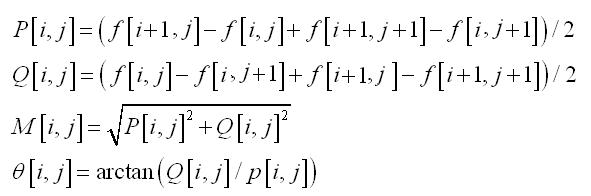
计算公式为:
其中$f$为图像灰度值,$P[i,j]$代表$[i,j]$在$X$方向梯度幅值,$Q[i,j]$代表$[i,j]$在$Y$方向的梯度幅值,$M[i,j]$是该点幅值,$\theta[i,j]$是梯度方向,也就是角度。
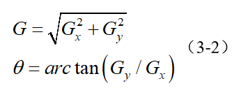
使用Sobel算子来计算梯度的大小及方向: 图像中的边缘可以指向各个方向,因此Canny算法使用四个算子来检测图像中的水平、垂直和对角边缘。边缘检测的算子(如Roberts,Prewitt,Sobel等)返回水平Gx和垂直Gy方向的一阶导数值,由此便可以确定像素点的梯度G和方向theta 。
其中G为梯度强度, theta表示梯度方向,arctan为反正切函数。下面以Sobel算子为例讲述如何计算梯度强度和方向。
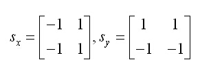
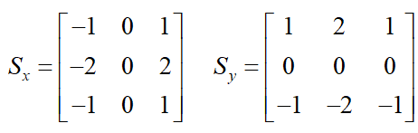
x和y方向的Sobel算子分别为:
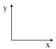
其中Sx表示x方向的Sobel算子,用于检测y方向的边缘; Sy表示y方向的Sobel算子,用于检测x方向的边缘(边缘方向和梯度方向垂直)。在直角坐标系中,Sobel算子的方向如下图所示。
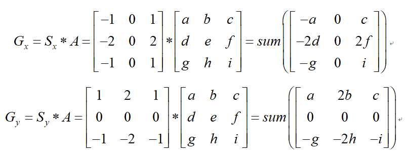
若图像中一个3x3的窗口为A,要计算梯度的像素点为e,则和Sobel算子进行卷积之后,像素点e在x和y方向的梯度值分别为:
其中*为卷积符号,sum表示矩阵中所有元素相加求和。根据公式(3-2)便可以计算出像素点e的梯度和方向。
下面是Sobel算子求梯度的java实现:
1
2
3
4
5
6
7
8
9
10
11
12
13
14
15
16
17
18
19
20
21
22
23
24
25
26
27
28
29
30
31
32
33
34
35
36
37
38
39
40
41
42
43
44
45
46
47
48
49
50
51
52
53
54
55
56
57
58
59
60
61
62
63
64
65
66
67
68
69
package edu.sfls.Jeff.JavaDev.CVLib;import org.opencv.core.Core;import org.opencv.core.CvType;import org.opencv.core.Mat;import java.util.concurrent.CountDownLatch;public class SmartSobel private Mat gradientX = new Mat(), gradientY = new Mat(), gradientXY = new Mat(); private double [][] pointDirection; public SmartSobel () public void compute (Mat image) throws InterruptedException pointDirection = new double [image.rows()][image.cols()]; for (int i = 0 ; i < image.rows(); i ++) for (int j = 0 ; j < image.cols(); j ++) pointDirection[i][j] = 0 ; gradientX = Mat.zeros(image.size(), CvType.CV_32SC1); gradientY = Mat.zeros(image.size(), CvType.CV_32SC1); gradientXY = Mat.zeros(image.size(), CvType.CV_32SC1); final CountDownLatch latch = new CountDownLatch(image.rows() - 2 ); for (int i = 1 ; i < image.rows() - 1 ; i ++) { int finalI = i; new Thread(() -> { for (int j = 1 ; j < image.cols() - 1 ; j++) { double gX = (-1 ) * image.get(finalI - 1 , j - 1 )[0 ] + 1 * image.get(finalI - 1 , j + 1 )[0 ] + (-2 ) * image.get(finalI, j - 1 )[0 ] + 2 * image.get(finalI, j + 1 )[0 ] + (-1 ) * image.get(finalI + 1 , j - 1 )[0 ] + 1 * image.get(finalI + 1 , j + 1 )[0 ]; double gY = 1 * image.get(finalI - 1 , j - 1 )[0 ] + 2 * image.get(finalI - 1 , j)[0 ] + 1 * image.get(finalI - 1 , j + 1 )[0 ] + (-1 ) * image.get(finalI + 1 , j - 1 )[0 ] + (-2 ) * image.get(finalI + 1 , j)[0 ] + (-1 ) * image.get(finalI + 1 , j + 1 )[0 ]; gradientY.put(finalI, j, Math.abs(gY)); gradientX.put(finalI, j, Math.abs(gX)); gradientXY.put(finalI, j, Math.sqrt(gX * gX + gY * gY)); if (gX == 0 ) gX = 0.00000000000000001 ; pointDirection[finalI][j] = Math.atan(gY / gX); } latch.countDown(); }).start(); } latch.await(); } public void convert () Core.convertScaleAbs(gradientX, gradientX); Core.convertScaleAbs(gradientY, gradientY); Core.convertScaleAbs(gradientXY, gradientXY); } public Mat getGradientX () return this .gradientX; } public Mat getGradientY () return this .gradientY; } public Mat getGradientXY () return this .gradientXY; } public double [][] getPointDirection() { return this .pointDirection; } }
由于这里使用的是$Math.tan()$,所以最终的角度是映射在$[-\frac \pi 2, \frac \pi 2]$的范围之内的。如果使用$Math.tan2()$会映射到$[-\pi,\pi]$的范围内,并且无需考虑符号影响,更加精确。但是这里我们并不关心另外的一个$\pi$的情况,我们只关心其所在直线(这在后文中会提到,也就是非极大值抑制),所以无需多考虑。
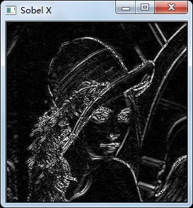
X方向梯度图:
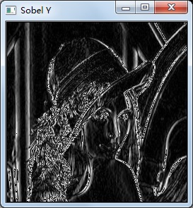
Y方向梯度图:
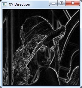
X、Y方向梯度融合效果:
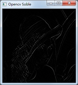
Opencv Sobel函数效果:
对梯度幅值进行非极大值抑制 非极大值抑制是一种边缘稀疏技术,非极大值抑制的作用在于“瘦”边。对图像进行梯度计算后,仅仅基于梯度值提取的边缘仍然很模糊。对于标准3,对边缘有且应当只有一个准确的响应。而非极大值抑制则可以帮助将局部最大值之外的所有梯度值抑制为0,对梯度图像中每个像素进行非极大值抑制的算法是:
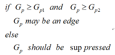
1) 将当前像素的梯度强度与沿正负梯度方向上的两个像素进行比较。
2) 如果当前像素的梯度强度与另外两个像素相比最大,则该像素点保留为边缘点,否则该像素点将被抑制。
通常为了更加精确的计算,在跨越梯度方向的两个相邻像素之间使用线性插值来得到要比较的像素梯度,现举例如下:
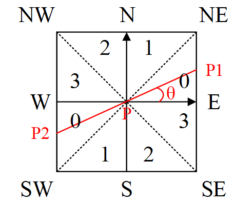
图3-2 梯度方向分割
如图3-2所示,将梯度分为8个方向,分别为E、NE、N、NW、W、SW、S、SE,其中0代表$0^\circ\sim45^\circ$,1代表$45^\circ\sim90^\circ$,2代表$-90^\circ\sim-45^\circ$,3代表$-45^\circ\sim0^\circ$。像素点P的梯度方向为$\theta$,则像素点P1和P2的梯度线性插值为:
上面也只是图中的情况,具体情况如下:
因此非极大值抑制的伪代码描写如下:
需要注意的是,如何标志方向并不重要,重要的是梯度方向的计算要和梯度算子的选取保持一致。
Java实现:
1
2
3
4
5
6
7
8
9
10
11
12
13
14
15
16
17
18
19
20
21
22
23
24
25
26
27
28
29
30
31
32
33
34
35
36
37
38
39
40
41
42
43
44
45
46
47
48
49
50
51
package edu.sfls.Jeff.JavaDev.CVLib;import org.opencv.core.CvType;import org.opencv.core.Mat;import java.util.concurrent.CountDownLatch;public class SmartNMS public static Mat NMS (Mat gradientImage, double [][] pointDirection) throws InterruptedException Mat outputImage = gradientImage.clone(); final CountDownLatch latch = new CountDownLatch(gradientImage.rows() - 2 ); for (int i = 1 ; i < gradientImage.rows() - 1 ; i ++) { int finalI = i; new Thread(() -> { for (int j = 1 ; j < gradientImage.cols() - 1 ; j ++) { double GP = gradientImage.get(finalI, j)[0 ], E = gradientImage.get(finalI, j + 1 )[0 ], NE = gradientImage.get(finalI - 1 , j + 1 )[0 ], N = gradientImage.get(finalI - 1 , j)[0 ], NW = gradientImage.get(finalI - 1 , j - 1 )[0 ], W = gradientImage.get(finalI, j - 1 )[0 ], SW = gradientImage.get(finalI + 1 , j - 1 )[0 ], S = gradientImage.get(finalI + 1 , j)[0 ], SE = gradientImage.get(finalI + 1 , j + 1 )[0 ]; double GP1 = 0 , GP2 = 0 ; double theta = pointDirection[finalI][j]; if (theta >= 0 && theta <= Math.PI / 4 ) { GP1 = E * (1 - Math.tan(theta)) + NE * Math.tan(theta); GP2 = W * (1 - Math.tan(theta)) + SW * Math.tan(theta); } else if (theta > Math.PI / 4 ) { GP1 = N * (1 - 1 / Math.tan(theta)) + NE * 1 / Math.tan(theta); GP2 = S * (1 - 1 / Math.tan(theta)) + SW * 1 / Math.tan(theta); } else if (theta < 0 && theta >= -Math.PI / 4 ) { GP1 = E * (1 - Math.tan(-theta)) + SE * Math.tan(-theta); GP2 = W * (1 - Math.tan(-theta)) + NW * Math.tan(-theta); } else { GP1 = S * (1 - 1 / Math.tan(-theta)) + SE * 1 / Math.tan(-theta); GP2 = N * (1 - 1 / Math.tan(-theta)) + NW * 1 / Math.tan(-theta); } if (GP < GP1 || GP < GP2) outputImage.put(finalI, j, 0 ); } latch.countDown(); }).start(); } latch.await(); return outputImage; } }
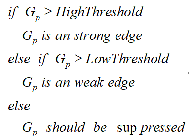
双阈值检测 在施加非极大值抑制之后,剩余的像素可以更准确地表示图像中的实际边缘。然而,仍然存在由于噪声和颜色变化引起的一些边缘像素。为了解决这些杂散响应,必须用弱梯度值过滤边缘像素,并保留具有高梯度值的边缘像素,可以通过选择高低阈值来实现。如果边缘像素的梯度值高于高阈值,则将其标记为强边缘像素;如果边缘像素的梯度值小于高阈值并且大于低阈值,则将其标记为弱边缘像素;如果边缘像素的梯度值小于低阈值,则会被抑制。阈值的选择取决于给定输入图像的内容。
双阈值检测的伪代码描写如下:
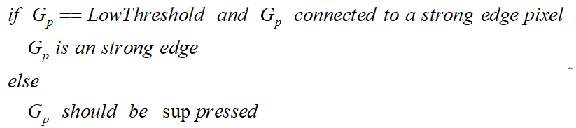
抑制孤立低阈值点 到目前为止,被划分为强边缘的像素点已经被确定为边缘,因为它们是从图像中的真实边缘中提取出来的。然而,对于弱边缘像素,将会有一些争论,因为这些像素可以从真实边缘提取也可以是因噪声或颜色变化引起的。为了获得准确的结果,应该抑制由后者引起的弱边缘。通常,由真实边缘引起的弱边缘像素将连接到强边缘像素,而噪声响应未连接。为了跟踪边缘连接,通过查看弱边缘像素及其8个邻域像素,只要其中一个为强边缘像素,则该弱边缘点就可以保留为真实的边缘。
抑制孤立边缘点的伪代码描述如下:
实现:(使用递归)
1
2
3
4
5
6
7
8
9
10
11
12
13
14
15
16
17
18
19
20
21
22
23
24
25
26
27
28
29
30
31
32
33
34
35
36
37
38
39
40
41
42
43
44
45
46
47
48
49
50
51
52
53
54
55
56
57
58
59
60
61
62
63
64
65
66
67
68
69
70
71
72
73
74
75
76
77
78
79
80
81
82
package edu.sfls.Jeff.JavaDev.CVLib;import org.opencv.core.Mat;import java.util.ArrayList;import java.util.List;public class SmartCanny private List<Integer[]> highPoints = new ArrayList<Integer[]>(); private void DoubleThreshold (Mat image, double lowThreshold, double highThreshold) for (int i = 1 ; i < image.rows() - 1 ; i ++) for (int j = 1 ; j < image.cols() - 1 ; j ++) if (image.get(i, j)[0 ] >= highThreshold) { image.put(i, j, 255 ); Integer[] p = new Integer[2 ]; p[0 ] = i; p[1 ] = j; highPoints.add(p); } else if (image.get(i, j)[0 ] < lowThreshold) image.put(i, j, 0 ); } private void DoubleThresholdLink (Mat image, double lowThreshold) for (Integer[] p : highPoints) { DoubleThresholdLinkRecurrent(image, lowThreshold, p[0 ], p[1 ]); } for (int i = 1 ; i < image.rows() - 1 ; i ++) for (int j = 1 ; j < image.cols() - 1 ; j ++) if (image.get(i, j)[0 ] < 255 ) image.put(i, j, 0 ); } private void DoubleThresholdLinkRecurrent (Mat image, double lowThreshold, int i, int j) if (i <= 0 || j <= 0 || i >= image.rows() - 1 || j >= image.cols() - 1 ) return ; if (image.get(i - 1 , j - 1 )[0 ] >= lowThreshold && image.get(i - 1 , j - 1 )[0 ] < 255 ) { image.put(i - 1 , j - 1 , 255 ); DoubleThresholdLinkRecurrent(image, lowThreshold, i - 1 , j - 1 ); } if (image.get(i - 1 , j)[0 ] >= lowThreshold && image.get(i - 1 , j)[0 ] < 255 ) { image.put(i - 1 , j, 255 ); DoubleThresholdLinkRecurrent(image, lowThreshold, i - 1 , j); } if (image.get(i - 1 , j + 1 )[0 ] >= lowThreshold && image.get(i - 1 , j + 1 )[0 ] < 255 ) { image.put(i - 1 , j + 1 , 255 ); DoubleThresholdLinkRecurrent(image, lowThreshold, i - 1 , j + 1 ); } if (image.get(i, j - 1 )[0 ] >= lowThreshold && image.get(i, j - 1 )[0 ] < 255 ) { image.put(i, j - 1 , 255 ); DoubleThresholdLinkRecurrent(image, lowThreshold, i, j - 1 ); } if (image.get(i, j + 1 )[0 ] >= lowThreshold && image.get(i, j + 1 )[0 ] < 255 ) { image.put(i, j + 1 , 255 ); DoubleThresholdLinkRecurrent(image, lowThreshold, i, j + 1 ); } if (image.get(i + 1 , j - 1 )[0 ] >= lowThreshold && image.get(i + 1 , j - 1 )[0 ] < 255 ) { image.put(i + 1 , j - 1 , 255 ); DoubleThresholdLinkRecurrent(image, lowThreshold, i + 1 , j - 1 ); } if (image.get(i + 1 , j)[0 ] >= lowThreshold && image.get(i + 1 , j)[0 ] < 255 ) { image.put(i + 1 , j, 255 ); DoubleThresholdLinkRecurrent(image, lowThreshold, i + 1 , j); } if (image.get(i + 1 , j + 1 )[0 ] >= lowThreshold && image.get(i + 1 , j + 1 )[0 ] < 255 ) { image.put(i + 1 , j + 1 , 255 ); DoubleThresholdLinkRecurrent(image, lowThreshold, i + 1 , j + 1 ); } } public Mat Canny (Mat image, int size, double sigma, double lowThreshold, double highThreshold) throws InterruptedException Mat tmp = SmartConverter.RGB2Gray((SmartGaussian.colorGaussianFilter(image, size, sigma))); SmartSobel ss = new SmartSobel(); ss.compute(tmp); ss.convert(); Mat ret = SmartNMS.NMS(ss.getGradientXY(), ss.getPointDirection()); this .DoubleThreshold(ret, lowThreshold, highThreshold); this .DoubleThresholdLink(ret, lowThreshold); return ret; } }
Reference [1] 高斯滤波及高斯卷积核C++实现 https://blog.csdn.net/dcrmg/article/details/52304446
[2] 边缘检测之Canny https://www.cnblogs.com/techyan1990/p/7291771.html
[3] Canny边缘检测及C++实现 https://blog.csdn.net/dcrmg/article/details/52344902
[4] Canny边缘检测算法 https://zhuanlan.zhihu.com/p/42122107
[5] Sobel算子及C++实现 https://blog.csdn.net/dcrmg/article/details/52280768

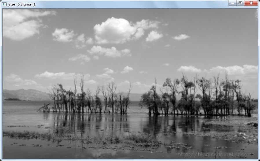 对比可以看到,Sigma(σ)越大,平滑效果越明显。