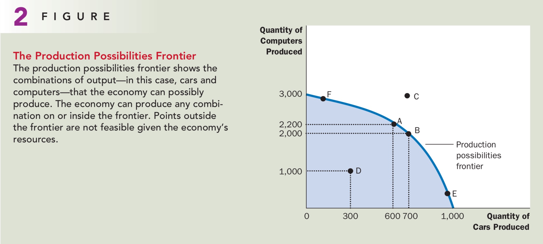
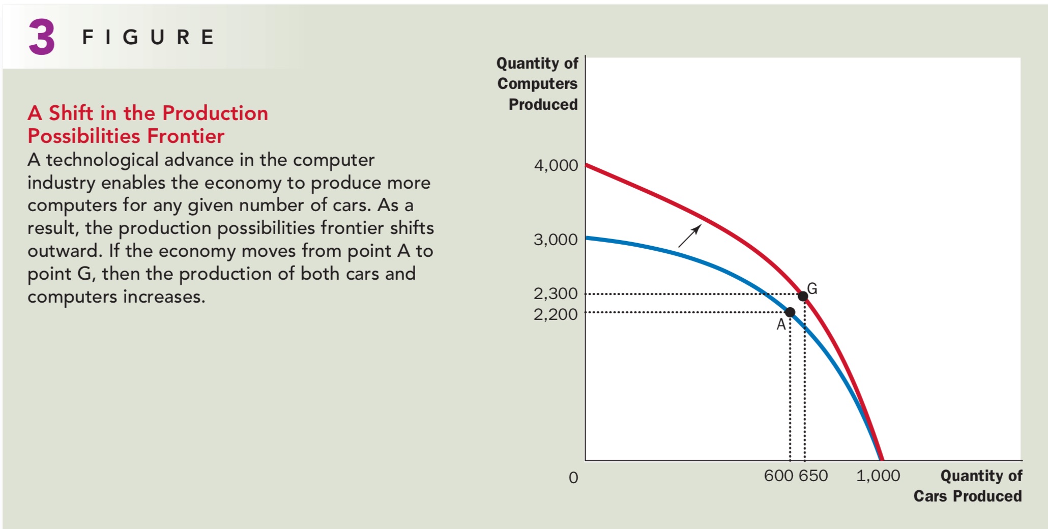
Production Possibility Frontier (PPF) - 生产可能性边界
- PPF 向外凸起
- 线上:Efficient,线外:Impossible,线内:Inefficient
Control on Prices - 价格管制
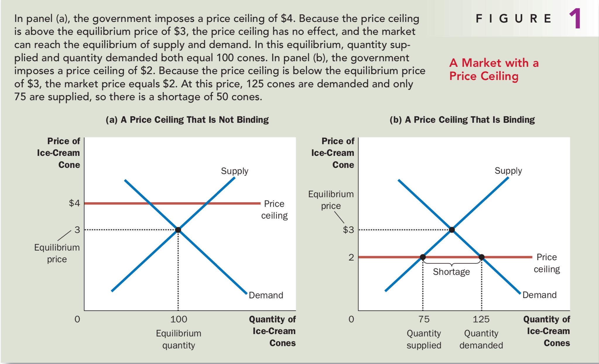
Price Ceiling - 价格天花板
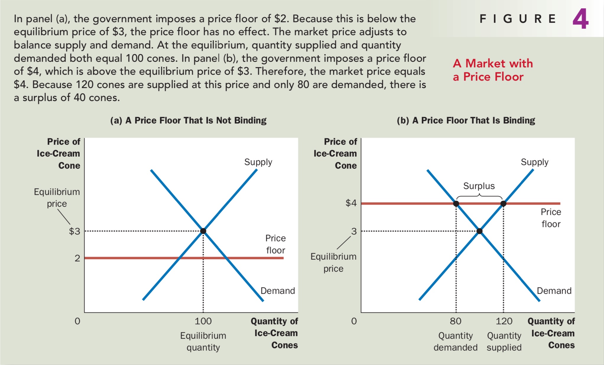
Price Floor - 价格地板
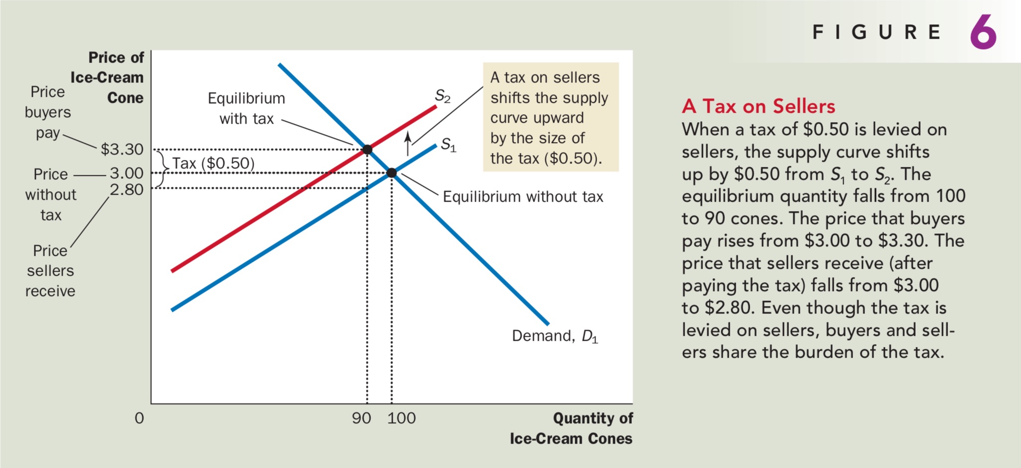
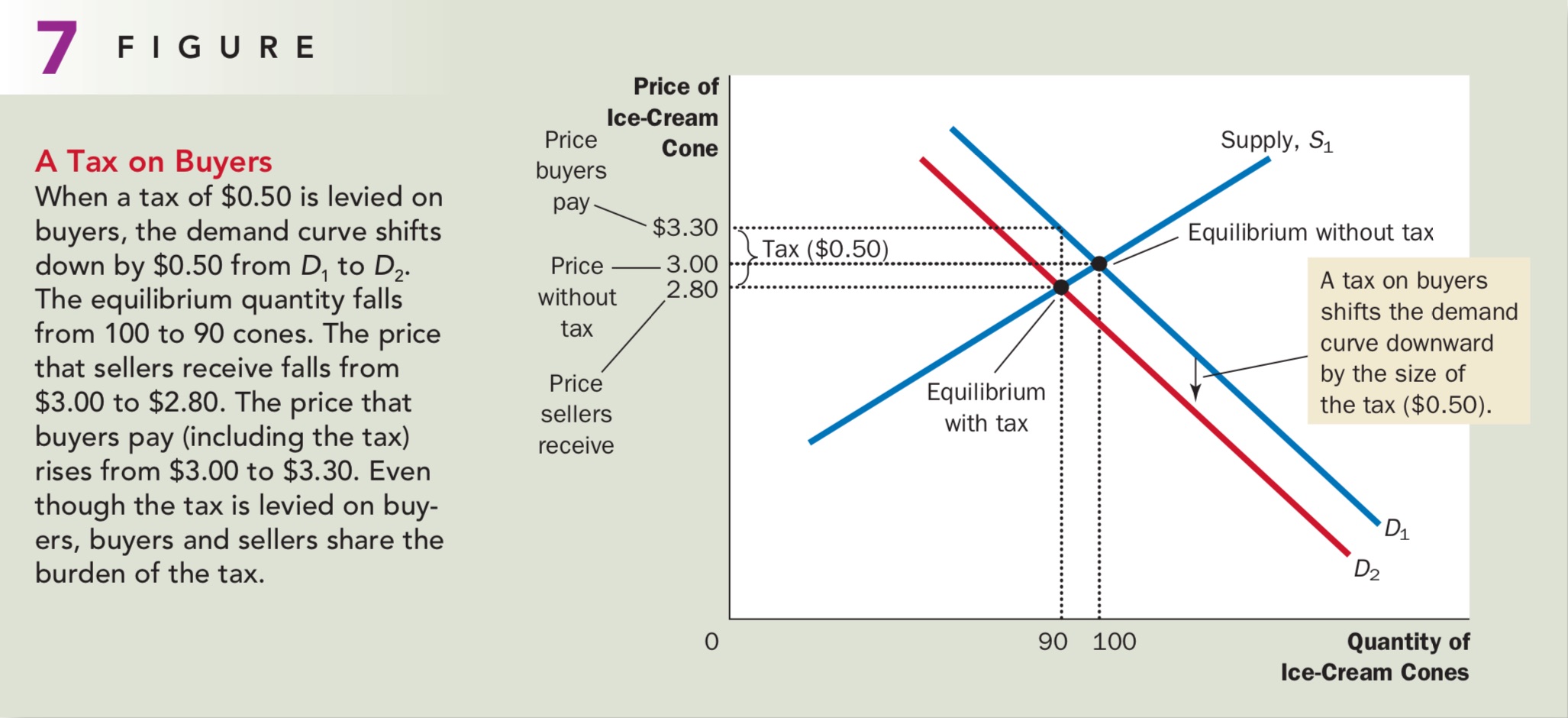
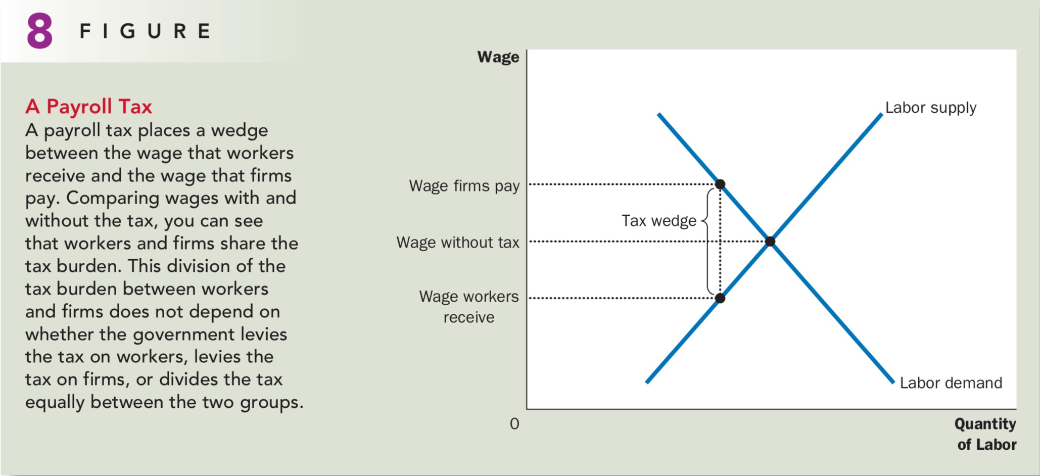
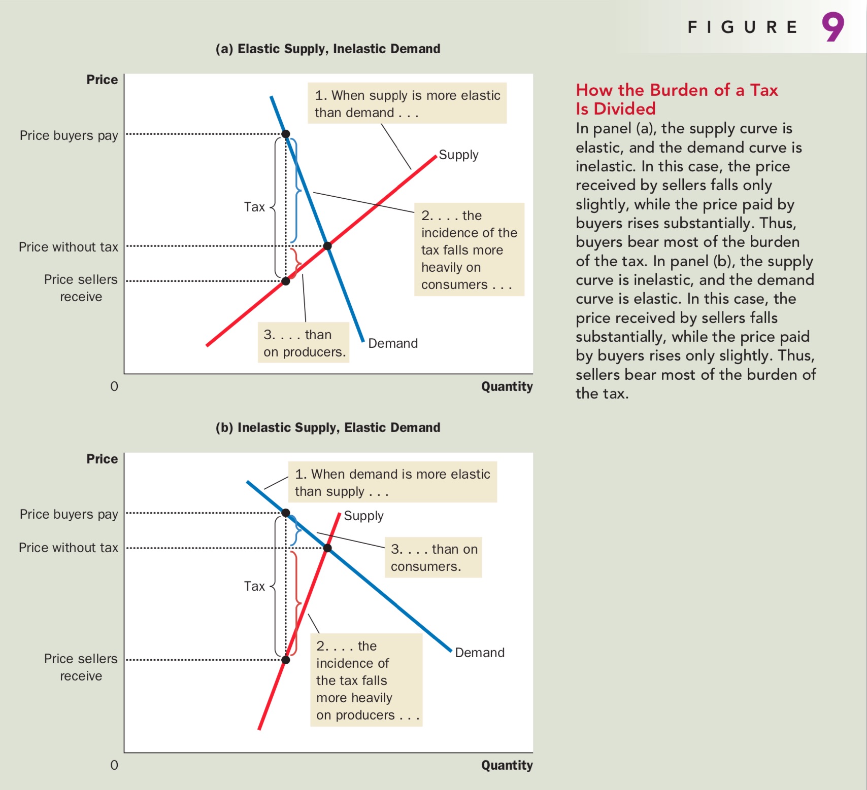
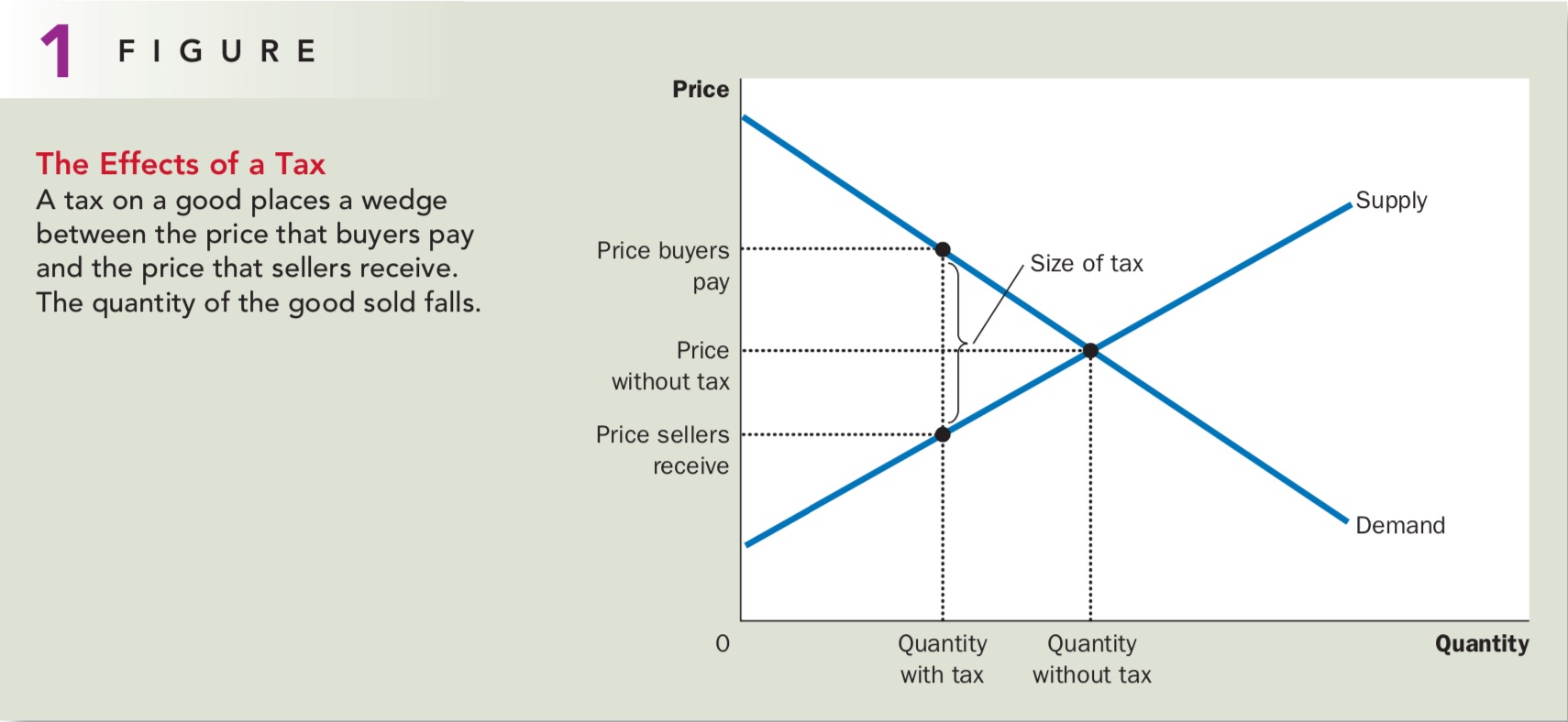
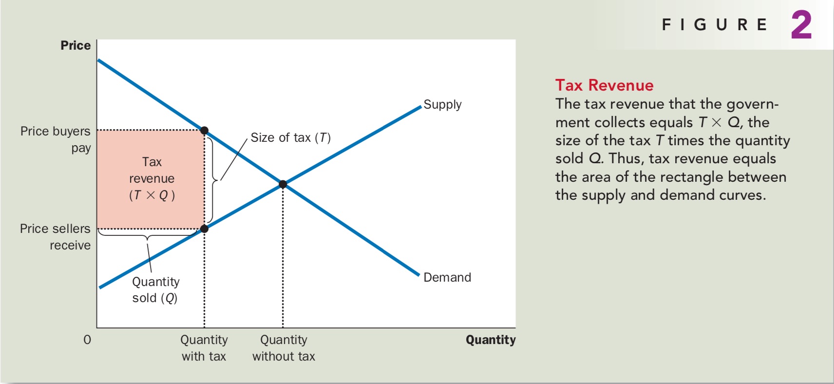
Taxation - 税收
结论2:可以通过税收wedge来计算
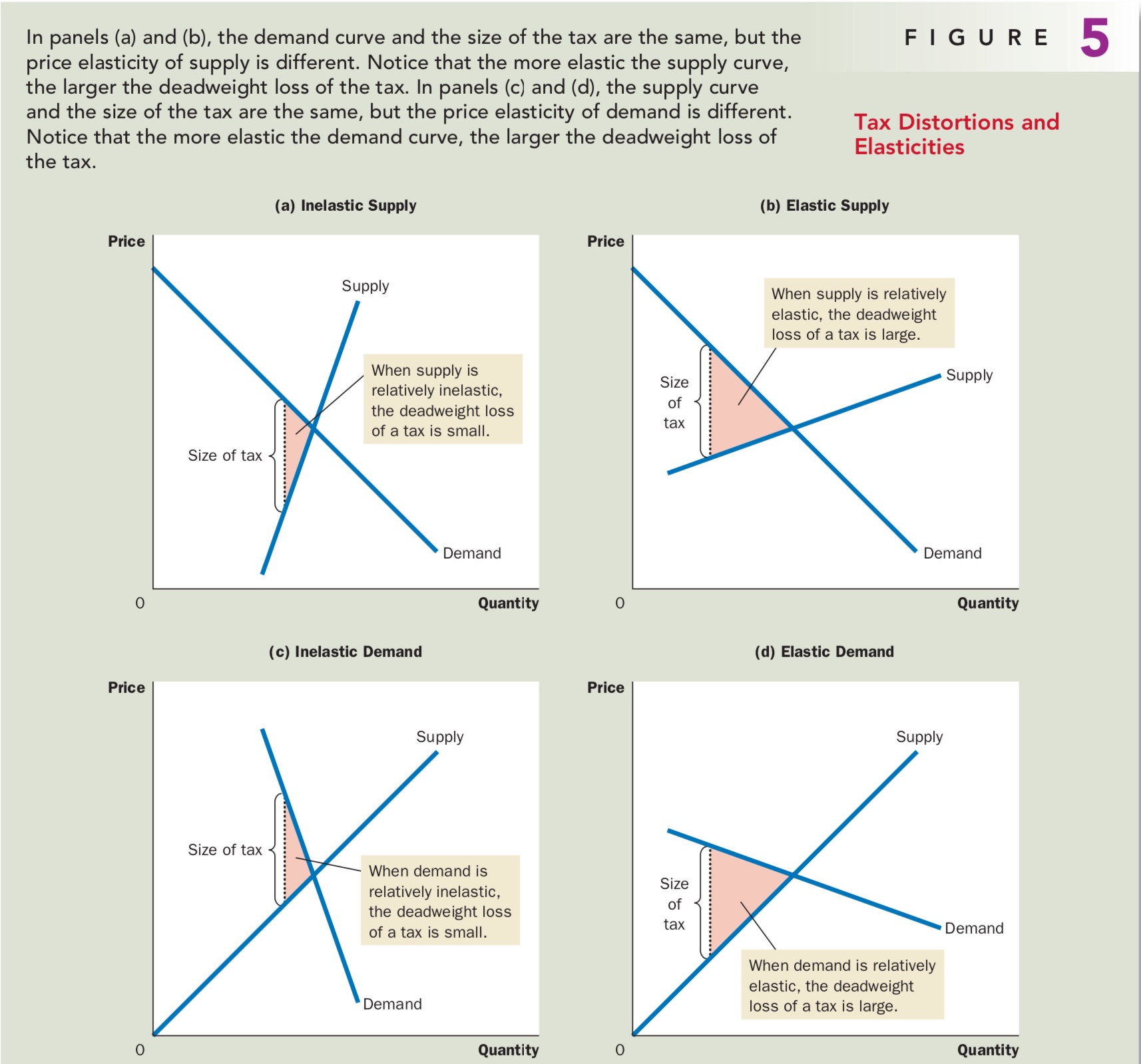
Elasticity - 弹性
弹性描述的是一个量对于另一个量变化的反应程度
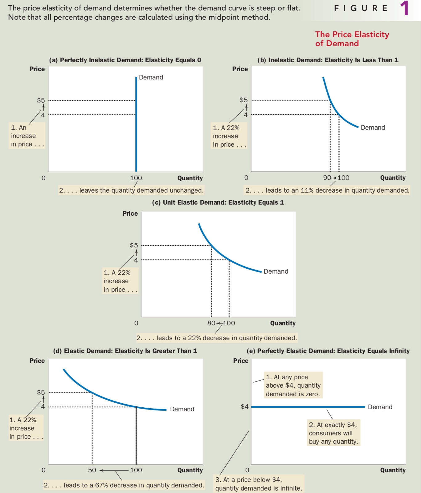
需求价格弹性
衡量某商品的需求量对其自身价格变动的反应程度
影响因素
- 相近商品的可得性 Availability of Cloase Substitues: 具有相近替代品的商品,一般需求弹性较大通俗理解:如果有替代品,你涨价,我就去买别人,所以这个对价格的变化需求量就会变化很大,所以弹性较大
- 必需品和奢侈品 Necessities versus Luxuries: 必需品(necessities)通常而言缺乏弹性,奢侈品(luxuries)通常富有弹性理解方法:刚需的弹性为零。奢侈品在涨价后,既然是奢侈品,那么可买可不买,所以奢侈品对价格的变动其需求量变化较大,弹性较大
- 市场的定义 Definition of the Market: 狭义市场比广义市场更有需求弹性理解方法:举个例子,如果要买纸巾:单一品牌纸巾的市场,相比于所有纸巾所构成的市场,弹性较大,因为整个市场需求量差不多是固定的,而一个品牌如果涨价,消费者就回去寻找替代品,这个和第一条规则类似
- 时间维度 Time Horizon: 某商品的长期需求通常比短期需求更加具有弹性理解方法:我加钱可以一点一点的涨,到头来还是要买
计算方法
衡量
- $\varepsilon > 1$ : Elastic
- $\varepsilon = 1$ : Unit Elasticity
- $\varepsilon < 1$ : Inelastic
- $\varepsilon \rightarrow \infty$ : Perfectly Elastic
- $\varepsilon = 0$ : Perfectly Inelastic
线性需求曲线
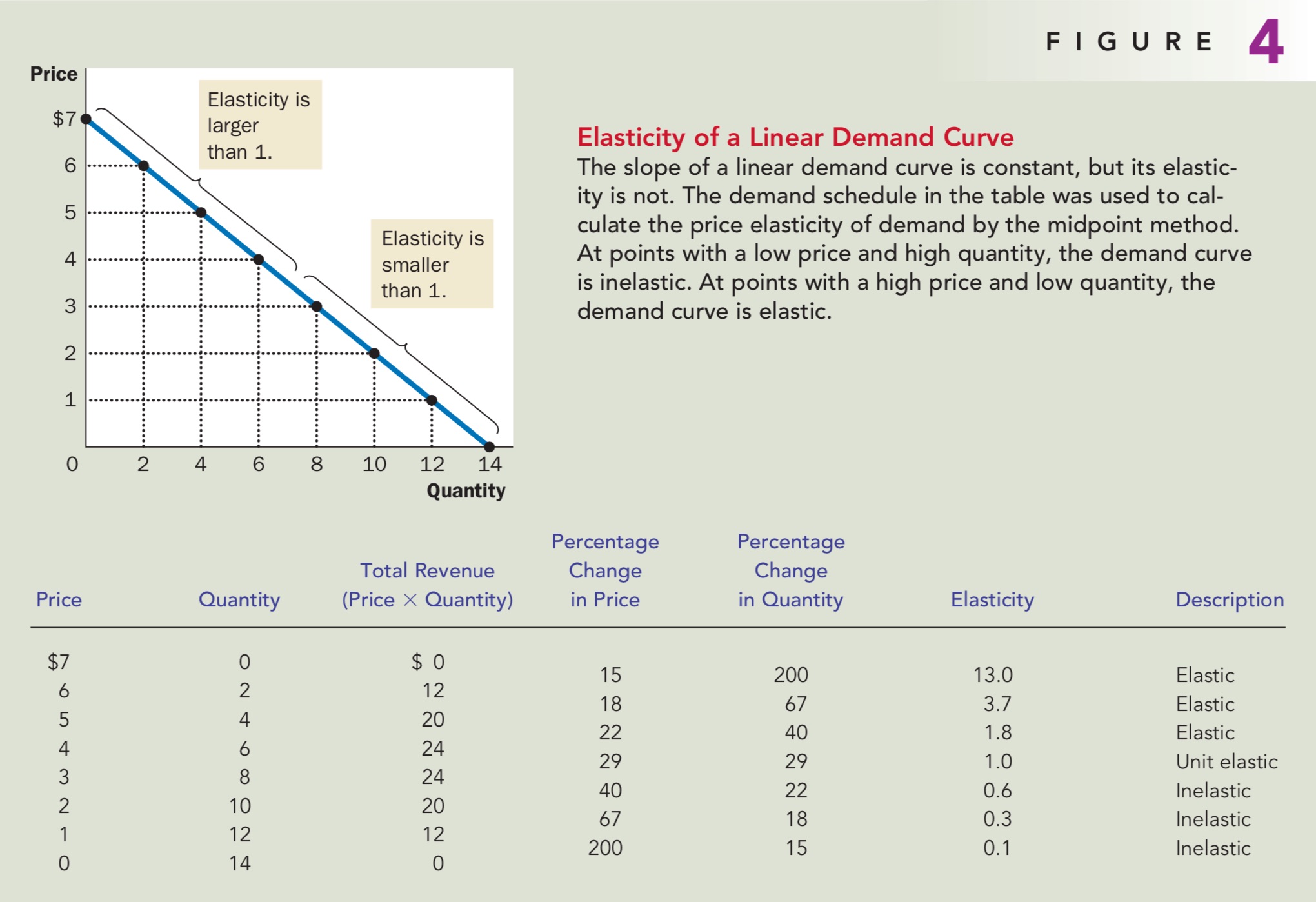
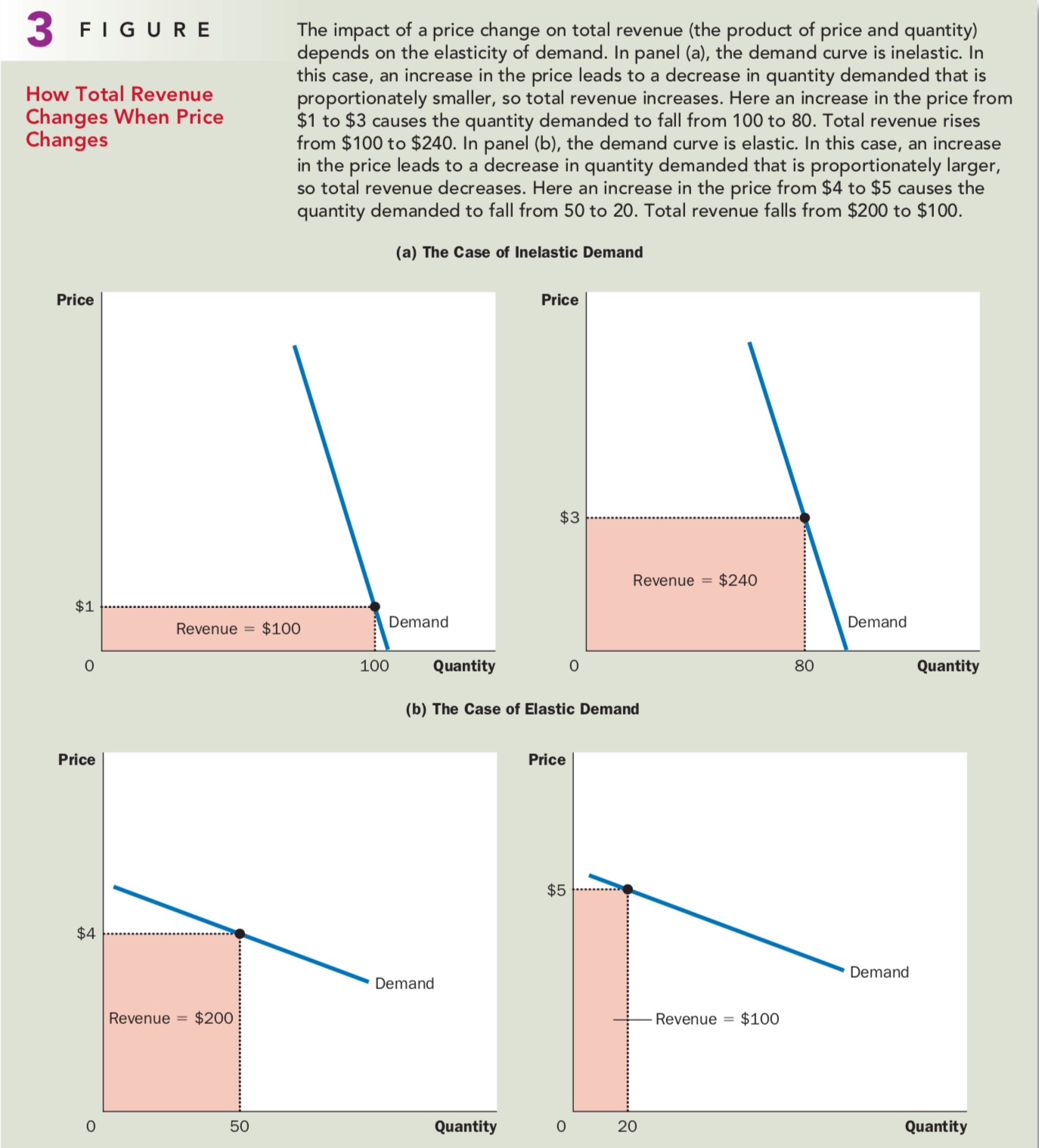
与Revenue之间的关系
对于Inelastic的商品
对于Elastic的商品
Welfare Economics - 福利经济学
消费者、生产者和市场的效率
重要概念
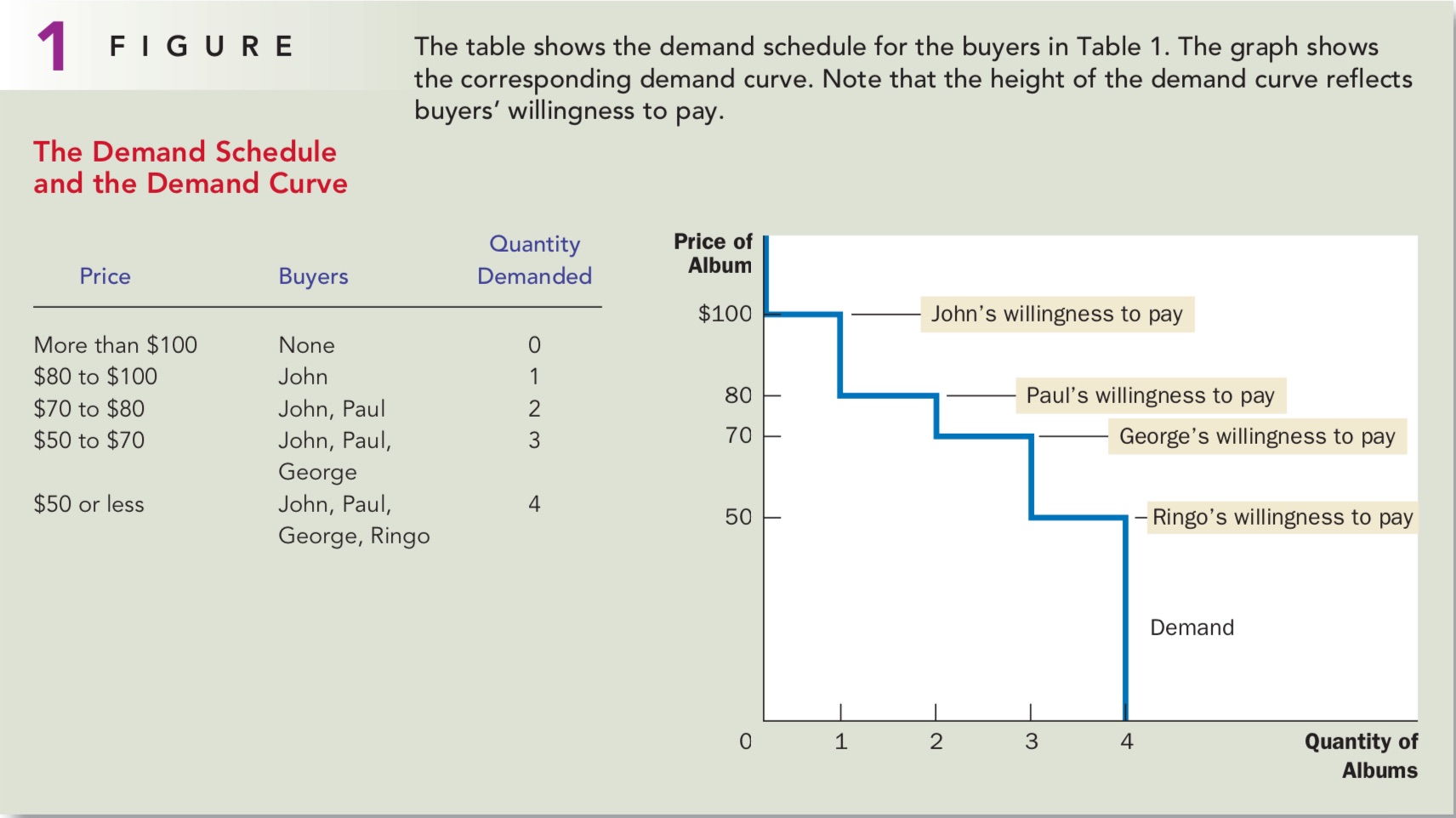
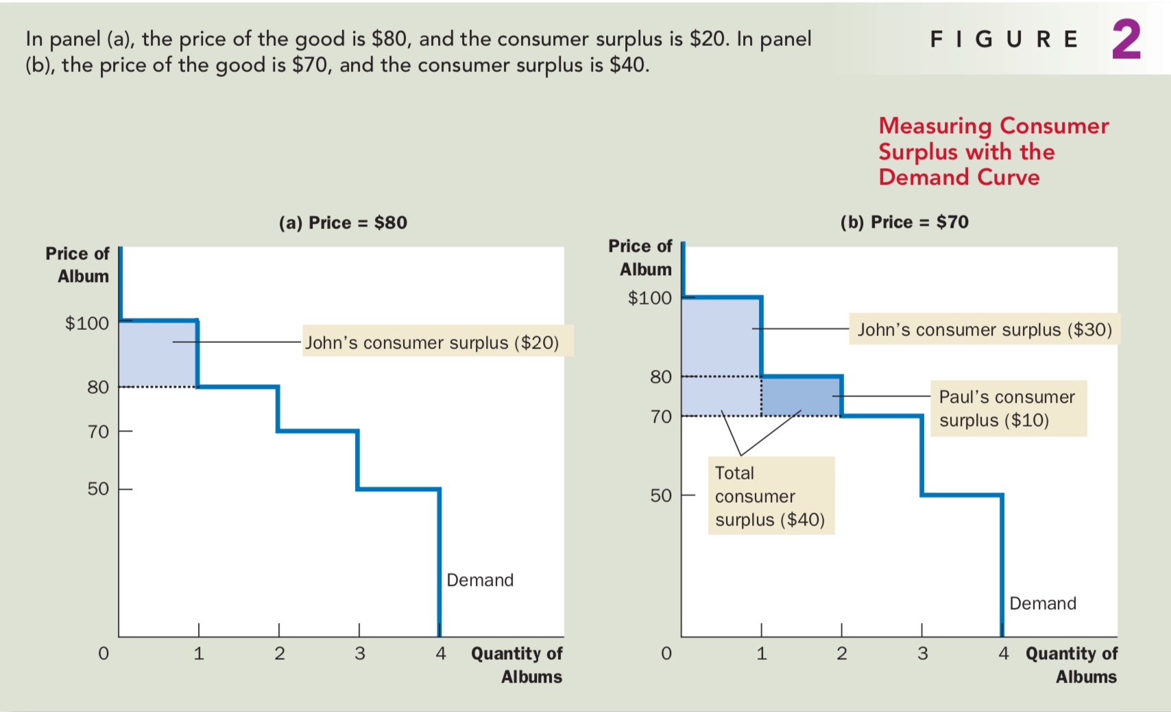
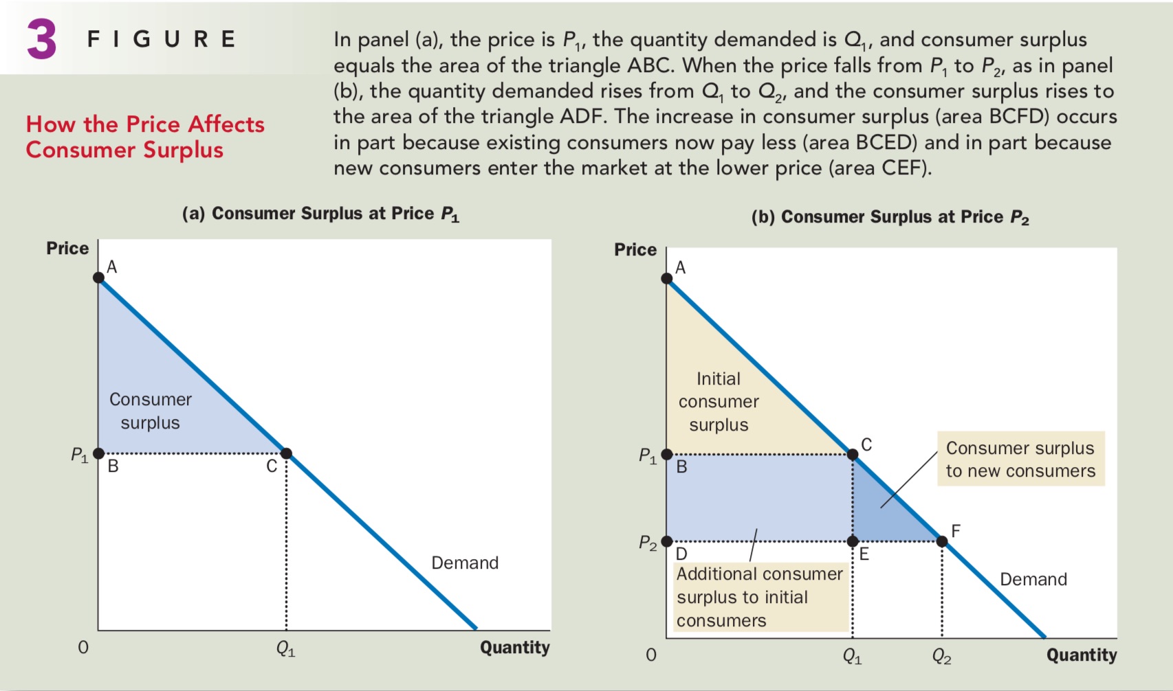
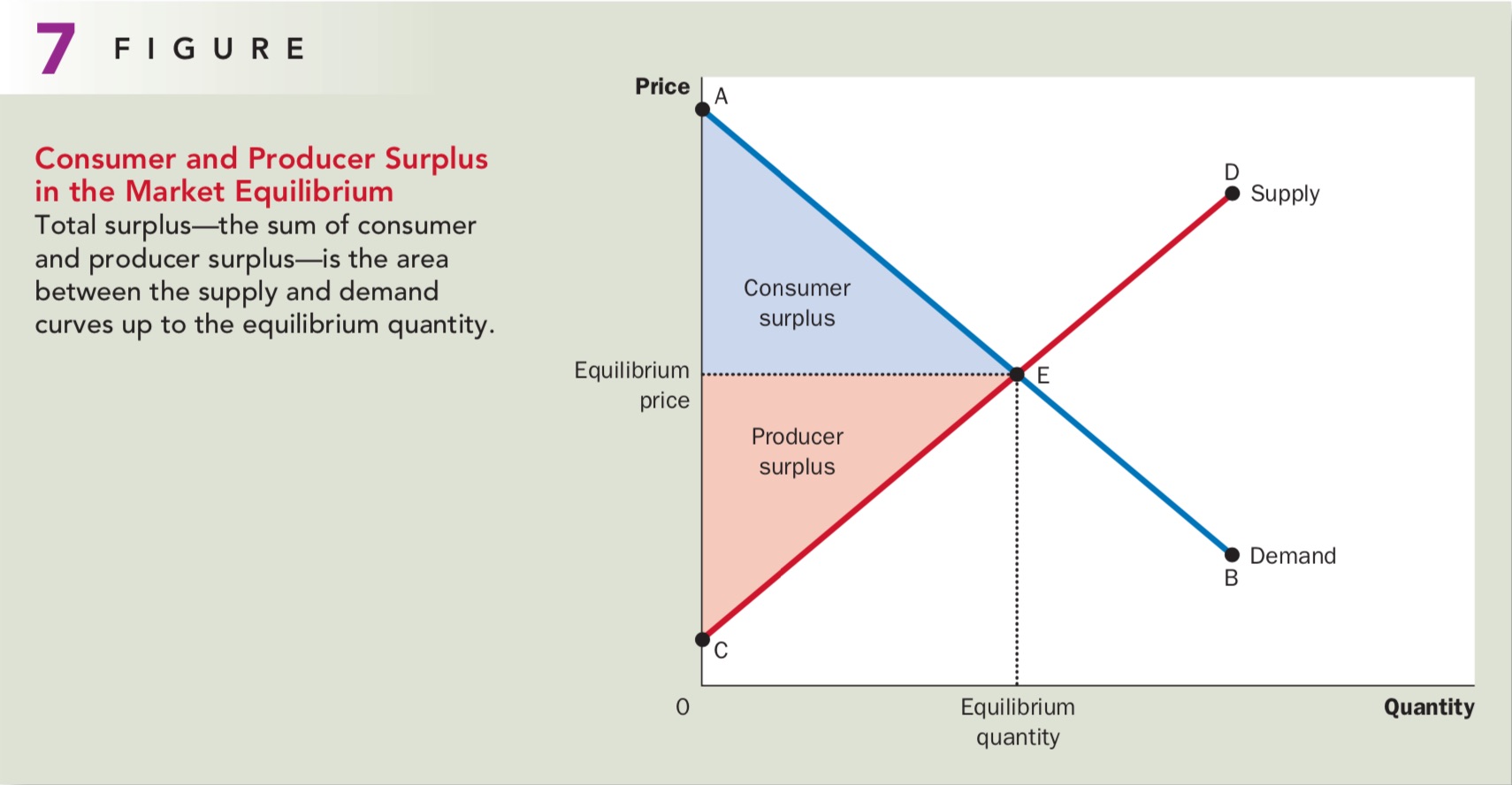
- Consumer Surplus = Value to buyers – Amount paid by buyers = 需求曲线之下,价格线之下的面积
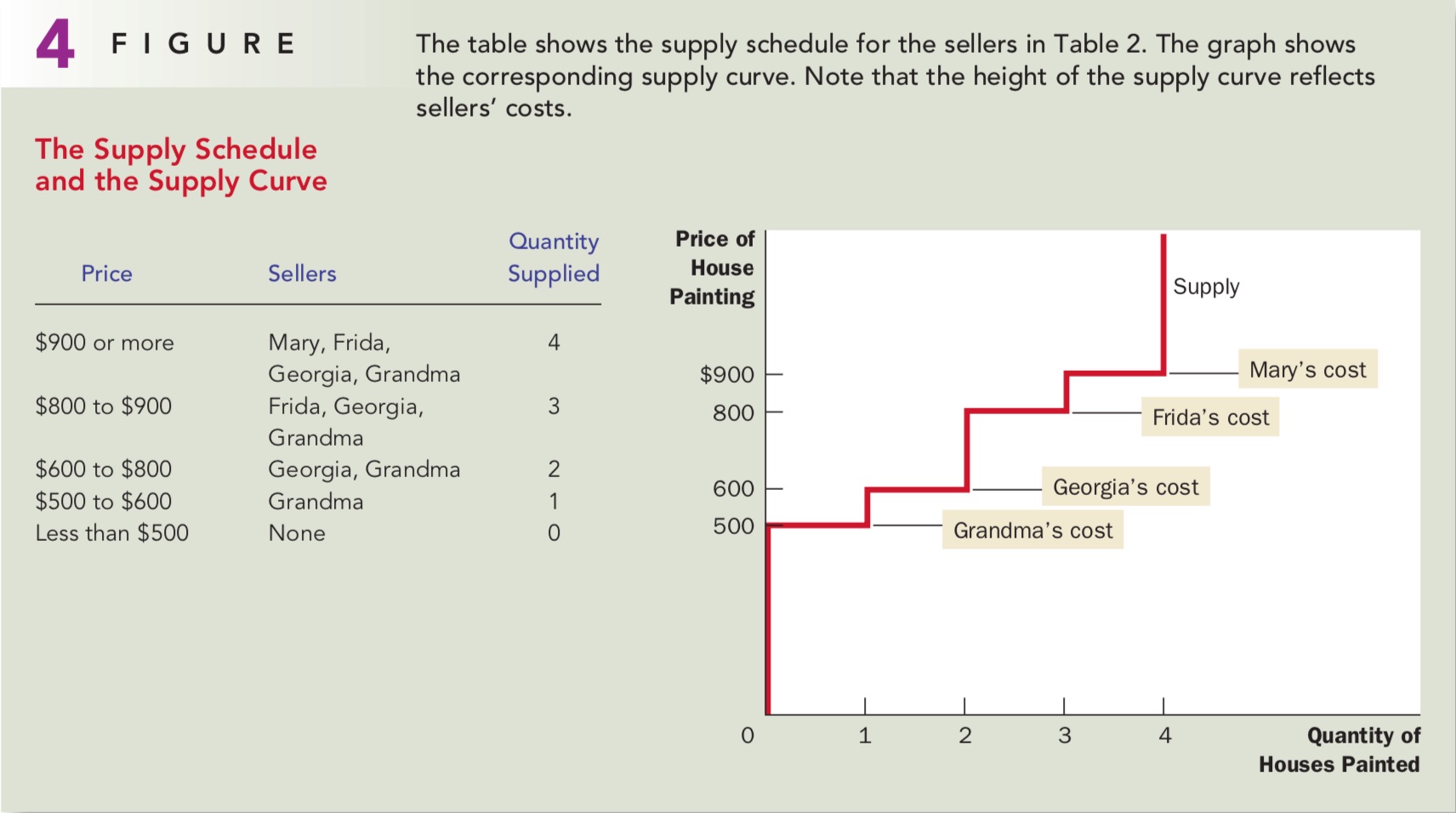
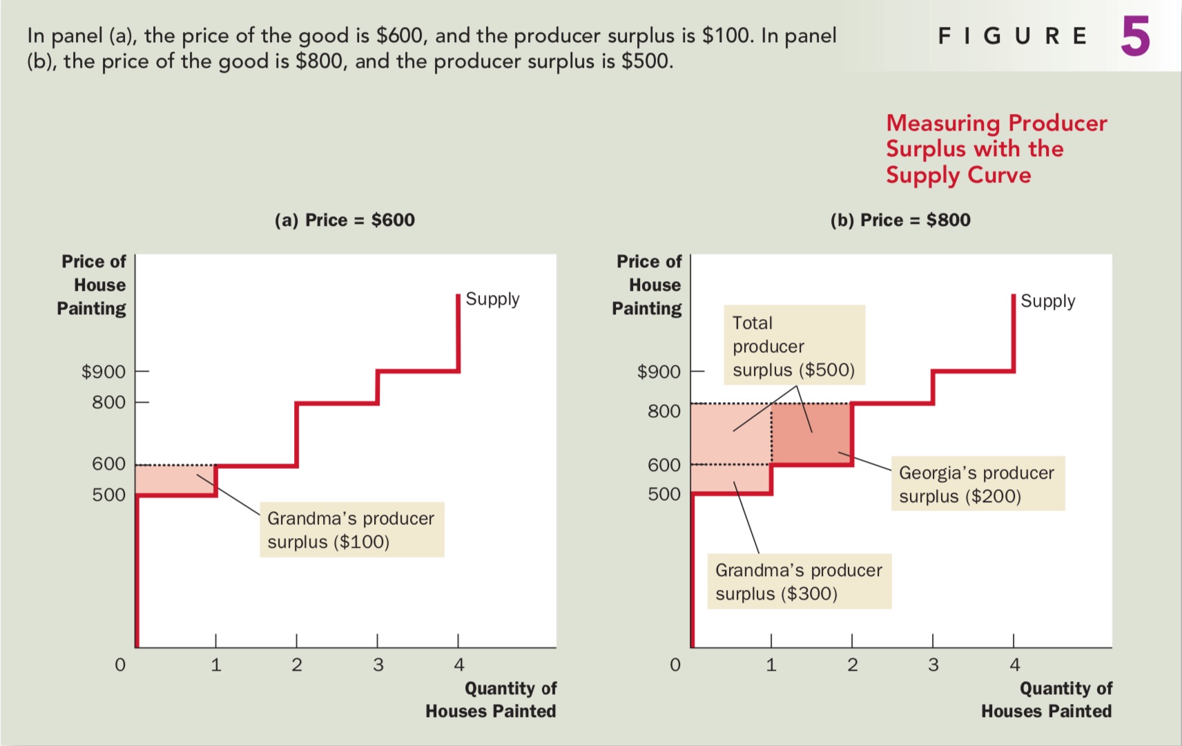
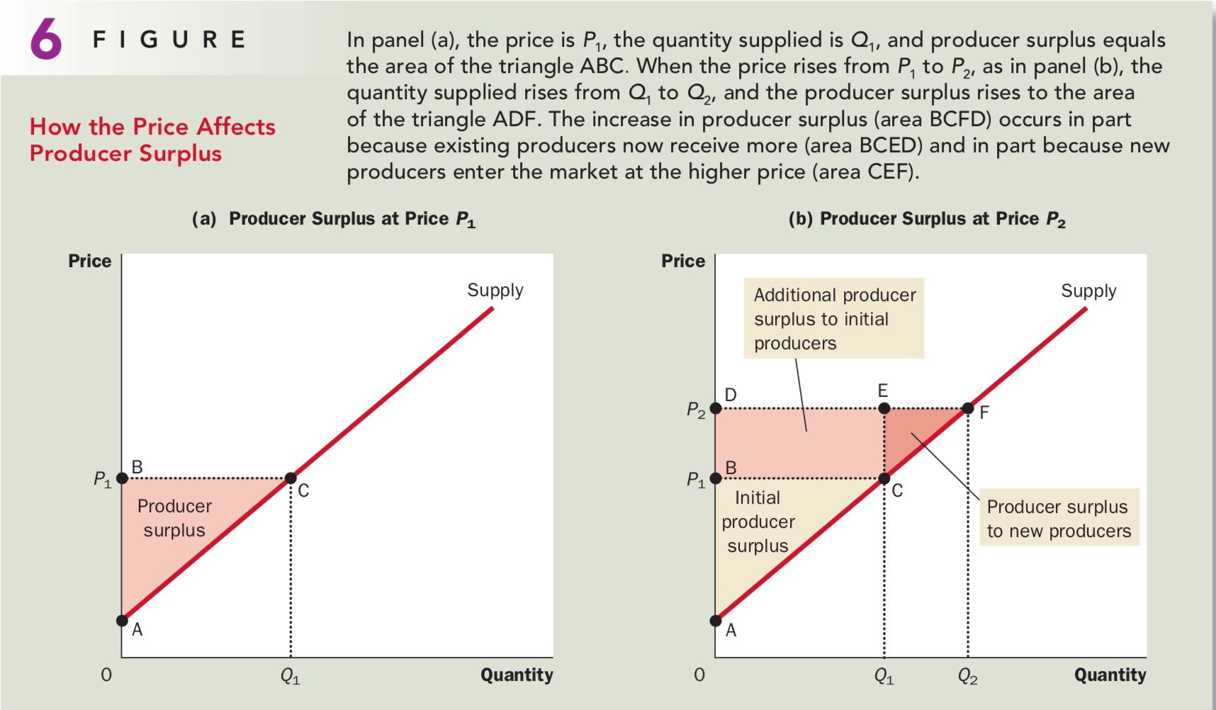
- Producer Surplus = Amount received by sellers – Cost to sellers = 供给曲线之上,价格线之下的面积
- Total Surplus = CS + PS = Willingness To Pay - Cost,体现市场效率
- 边际买者:价格提高后,第一个离开市场的人
- 边际卖者:价格下降后,第一个离开市场的人
图像
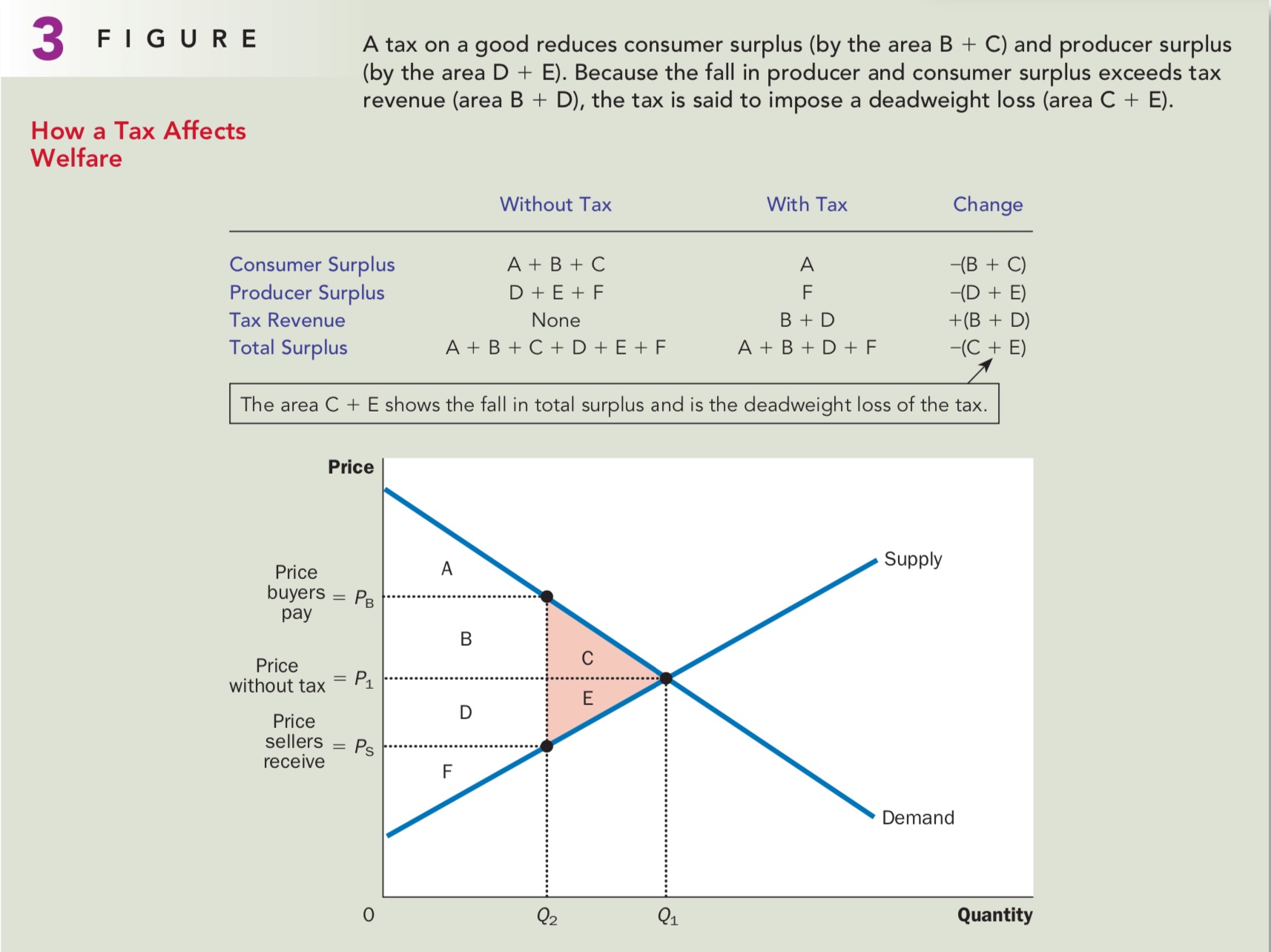
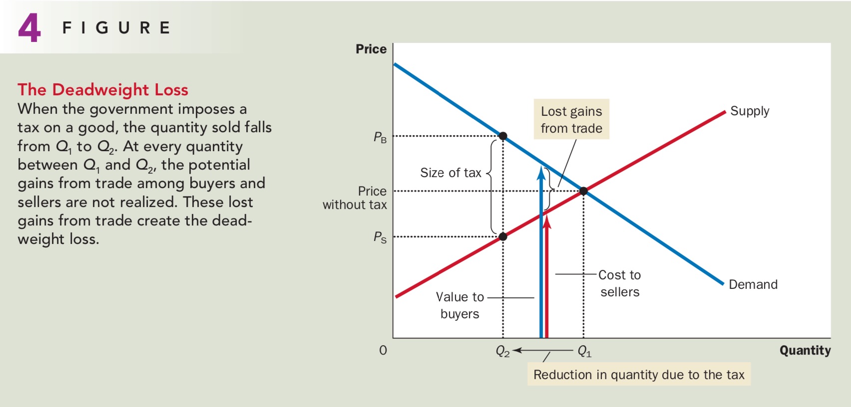
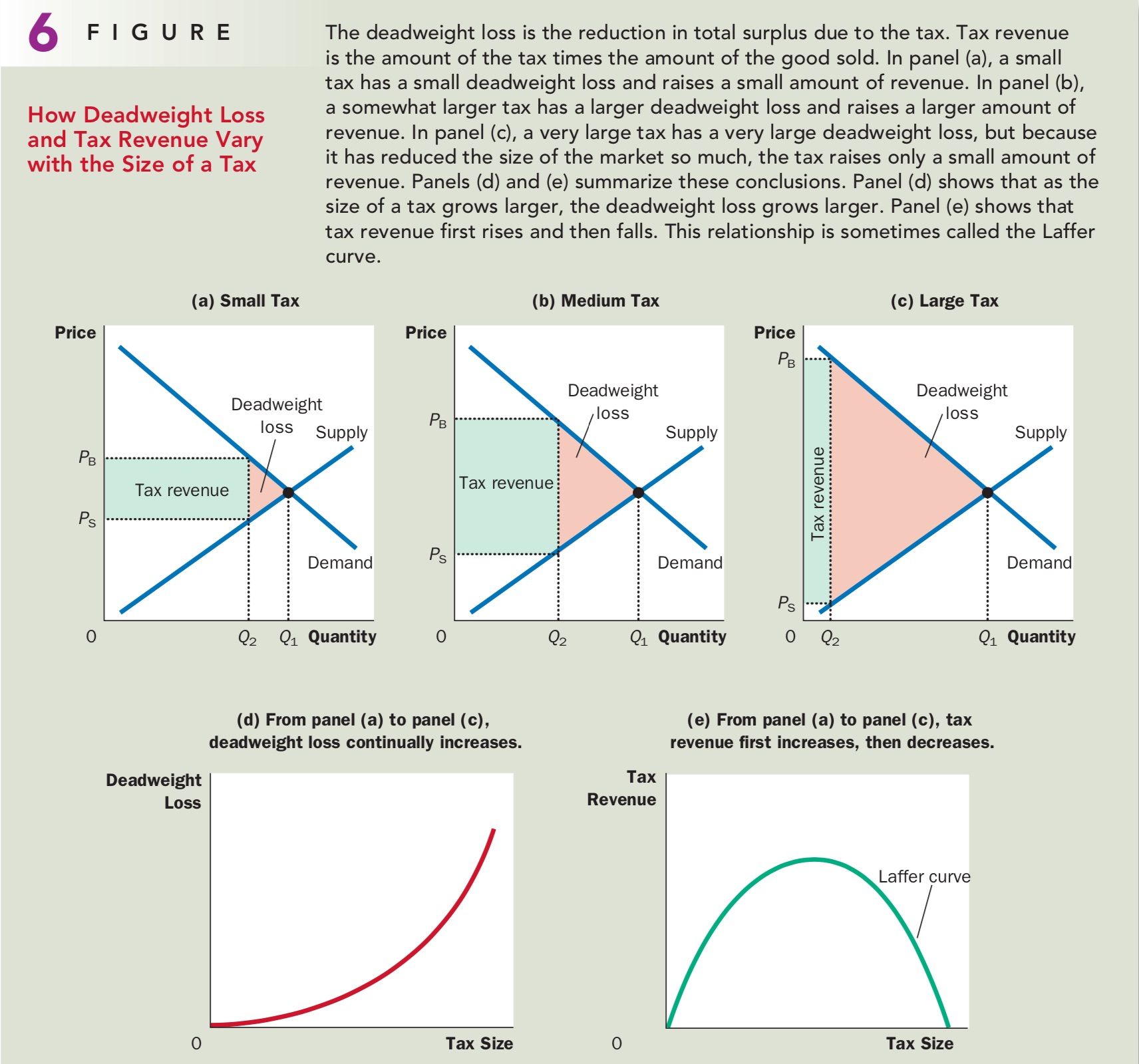
征税的代价 - 产生Deadweight Loss
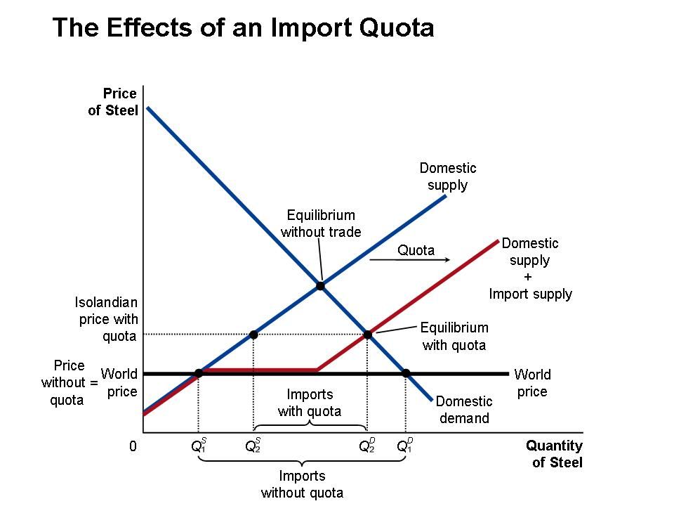
International Trade - 国际贸易
要点
- 开放国际贸易,就要接受国际的价格
- 如果World Price > Domestic Price,出口
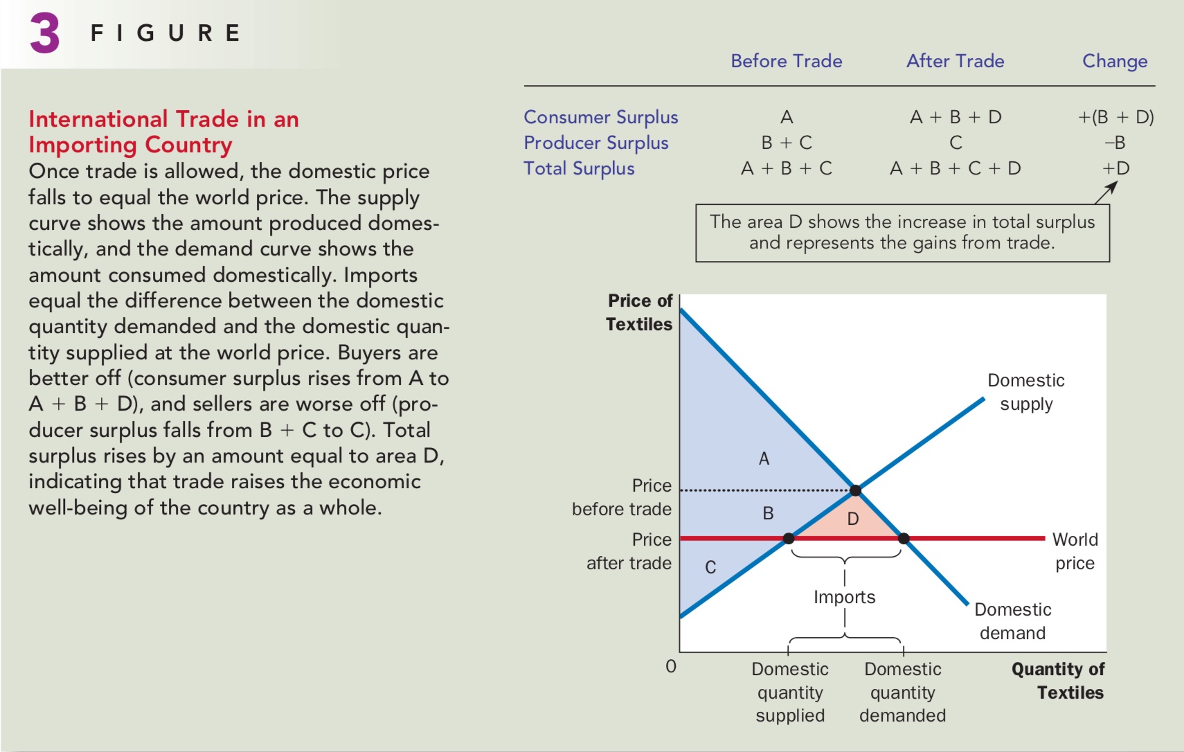
- 如果World Price < Domestic Price,进口
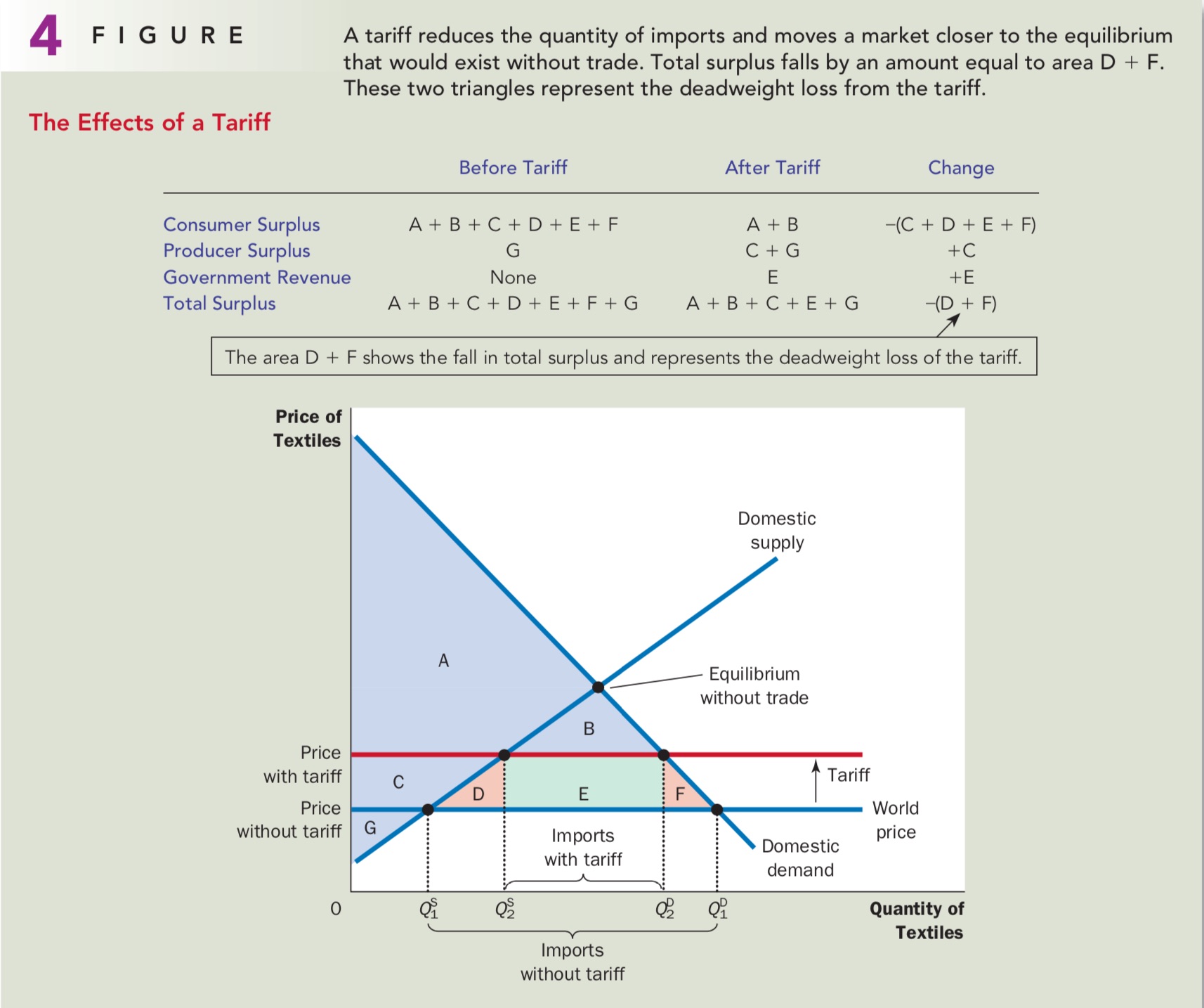
- Tariff有无谓损失,Quota没有
- Tariff政府拿得到钱,有Tax Revenue,Quota没有
国际贸易的图像
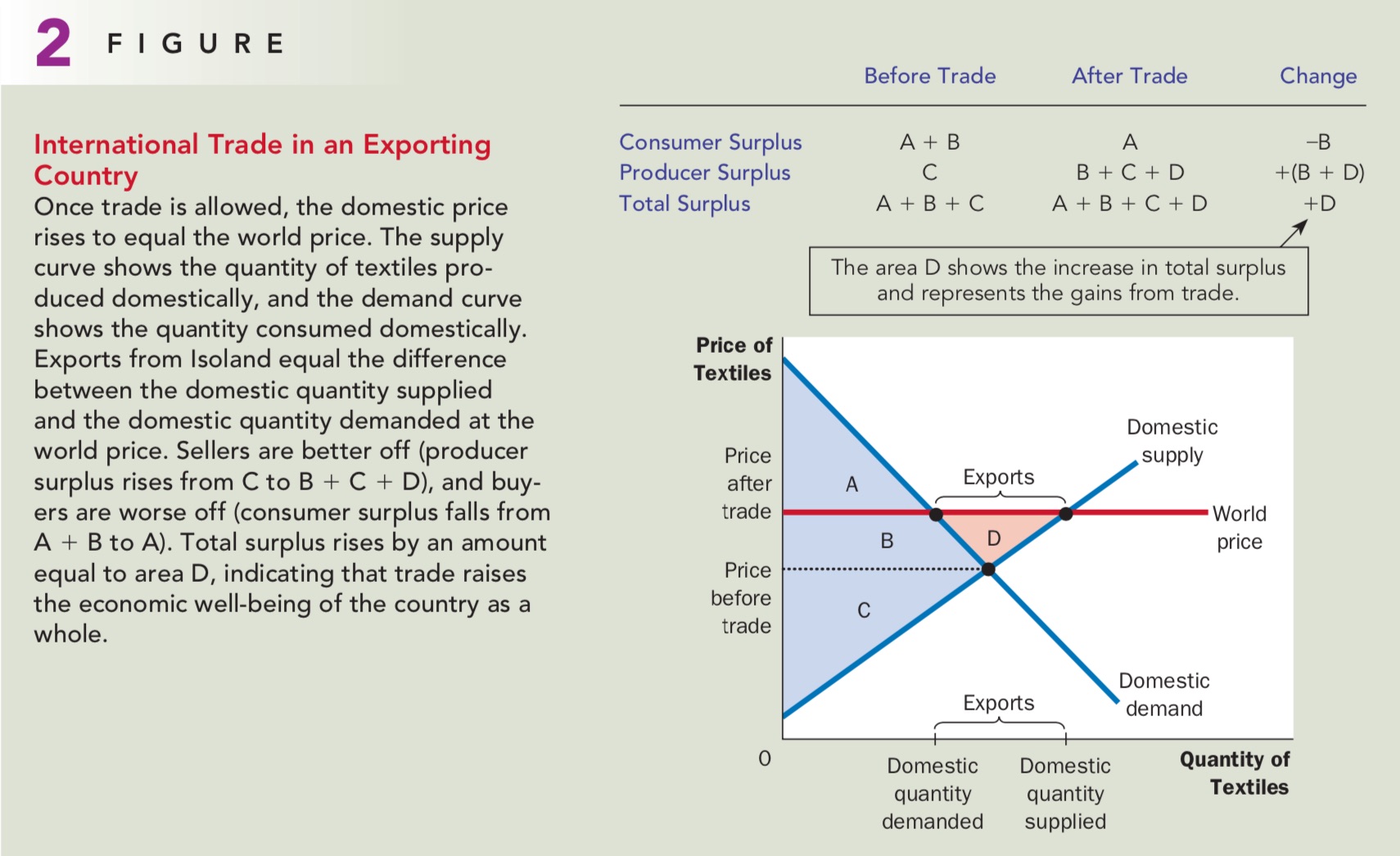
国际贸易的好处
- 商品多样性增加
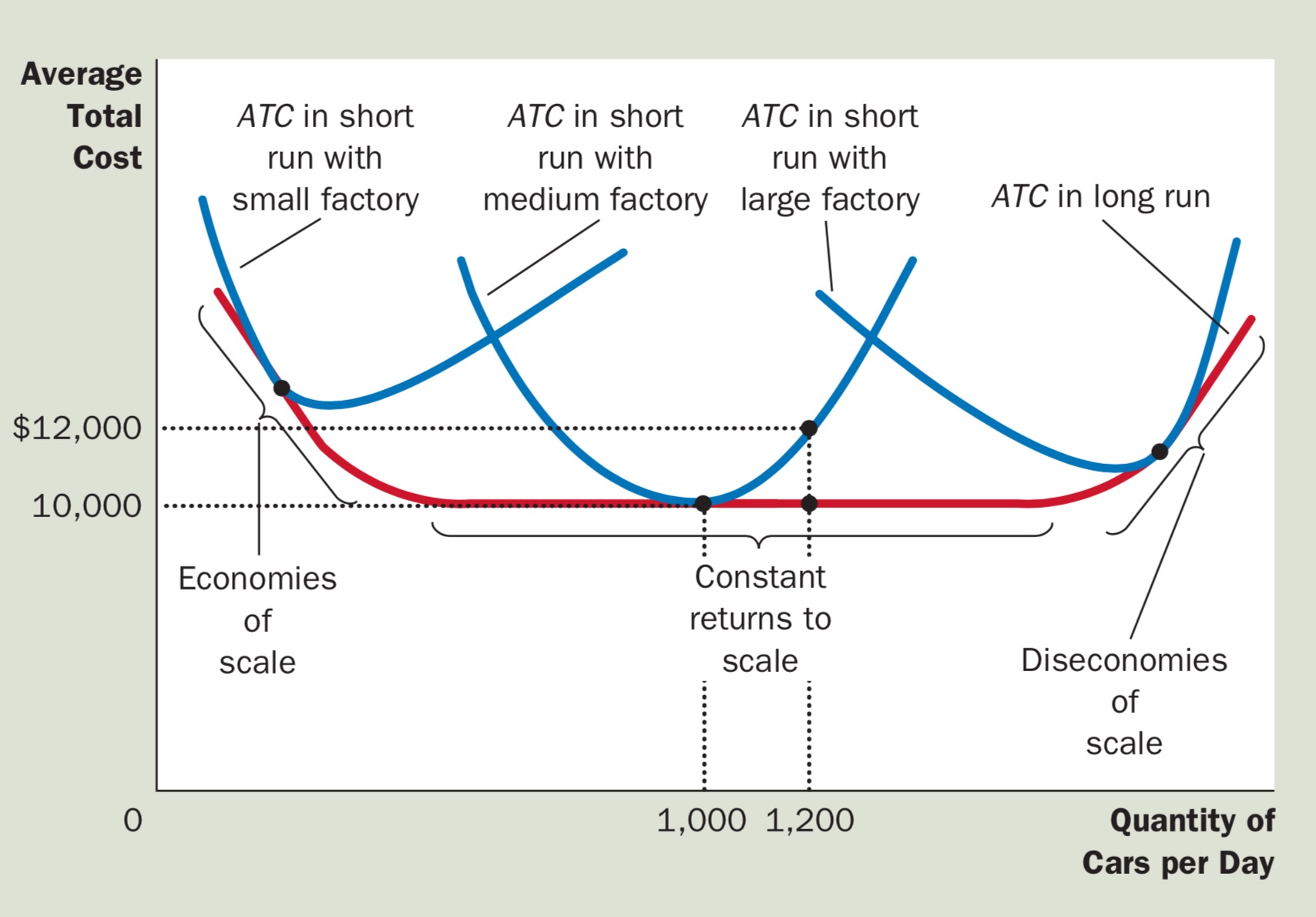
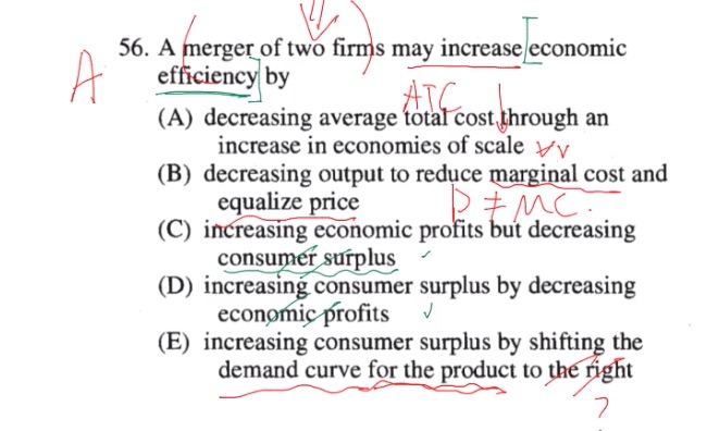
- 规模经济降低成本(economies of scale)
- 竞争程度增加
- 科技流动性增加
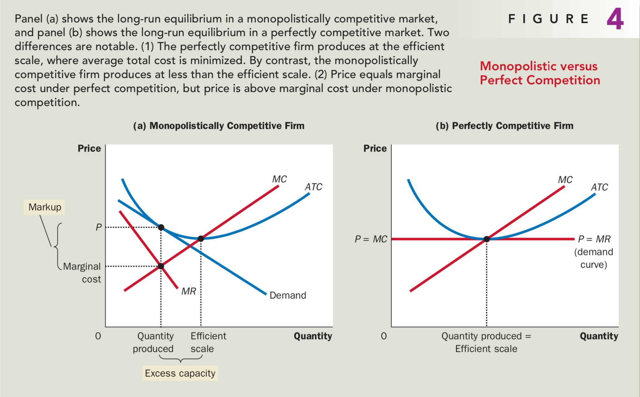
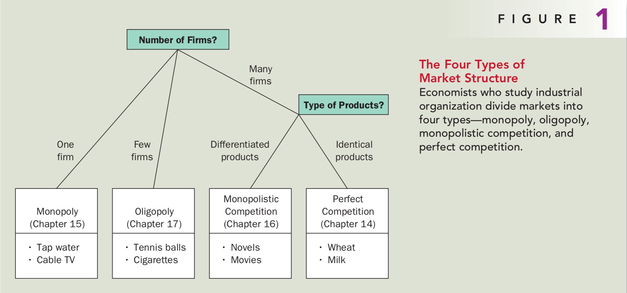
Perfectly Competitive Market - 完全竞争市场
完全竞争市场的特点
长期的价格不会改变,过程: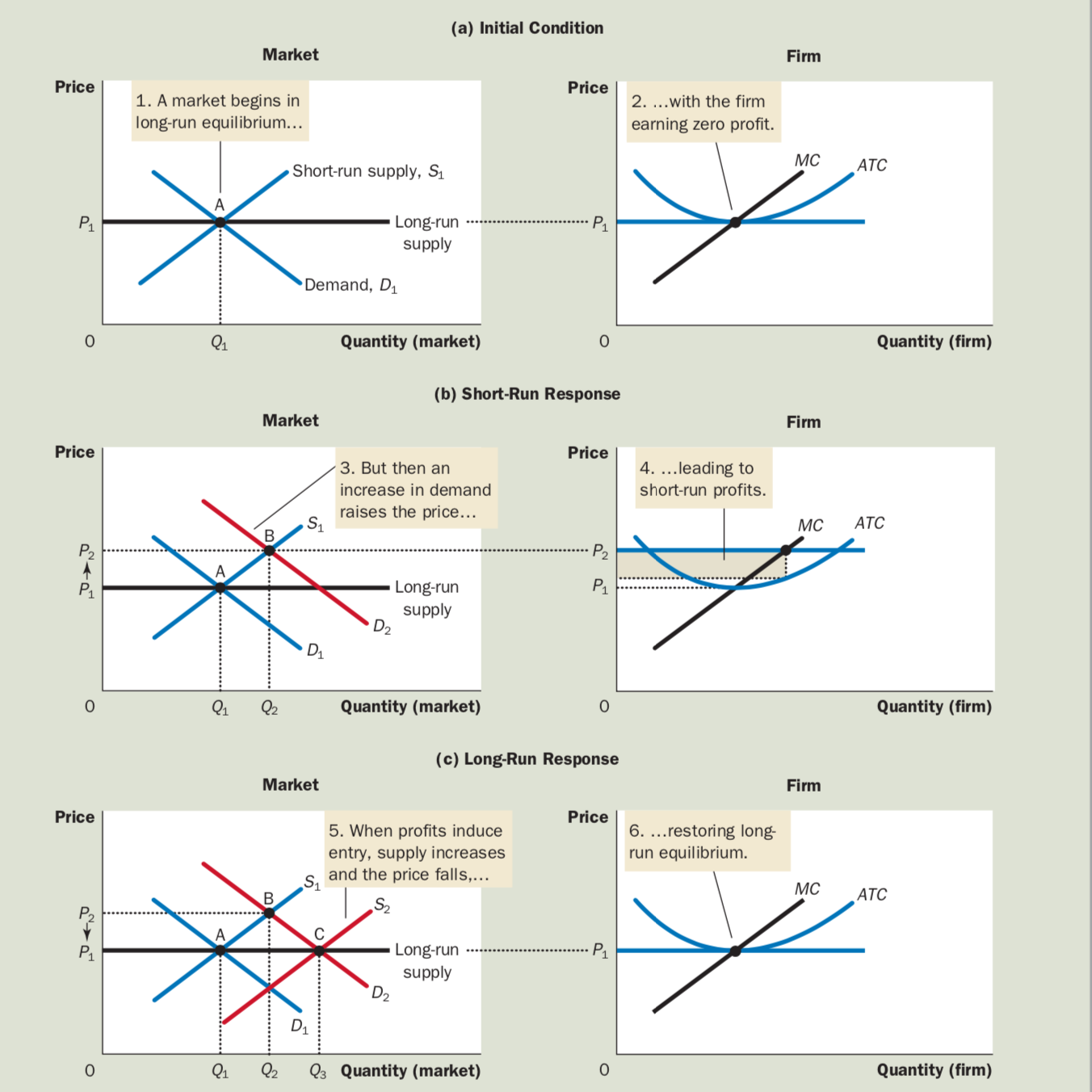
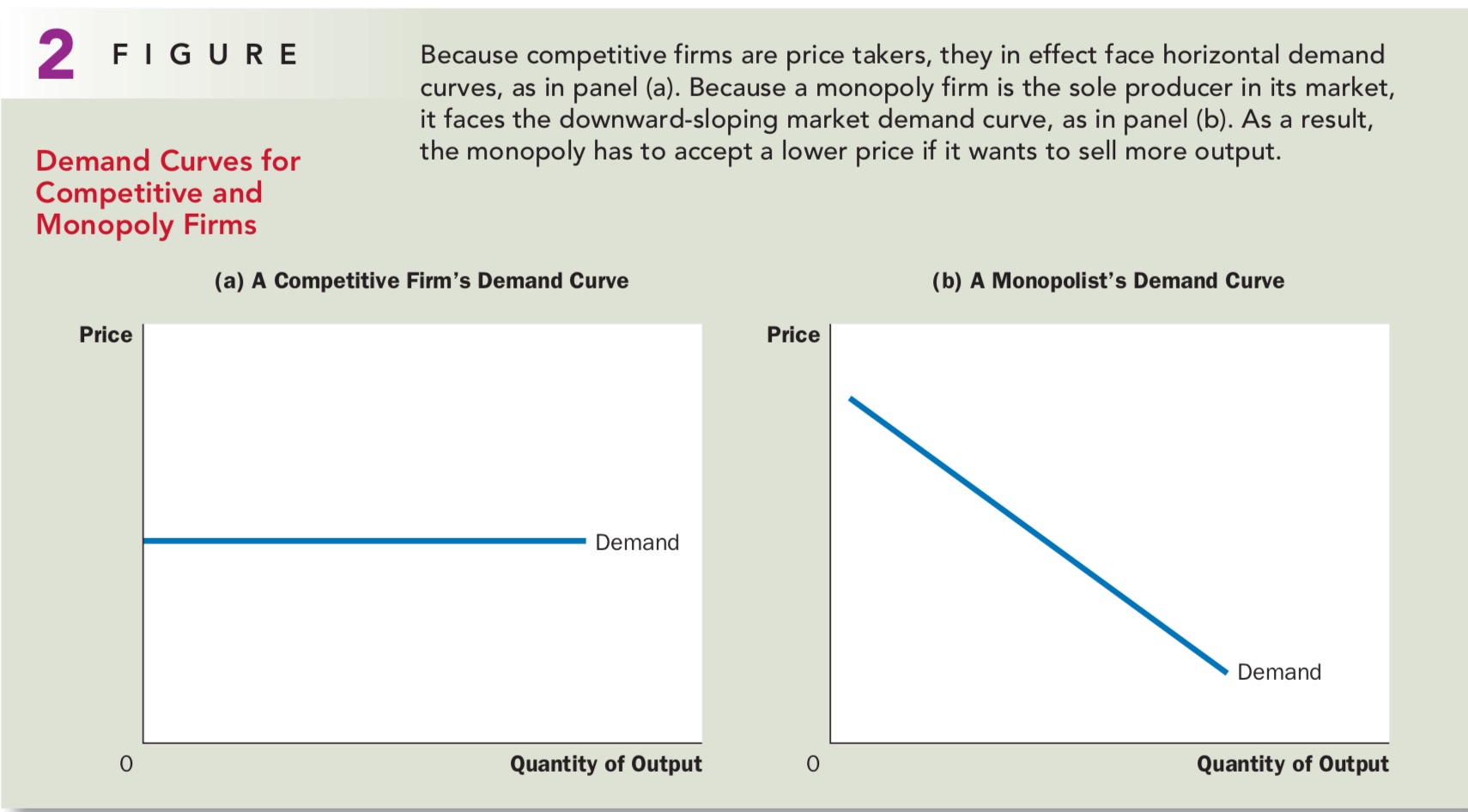
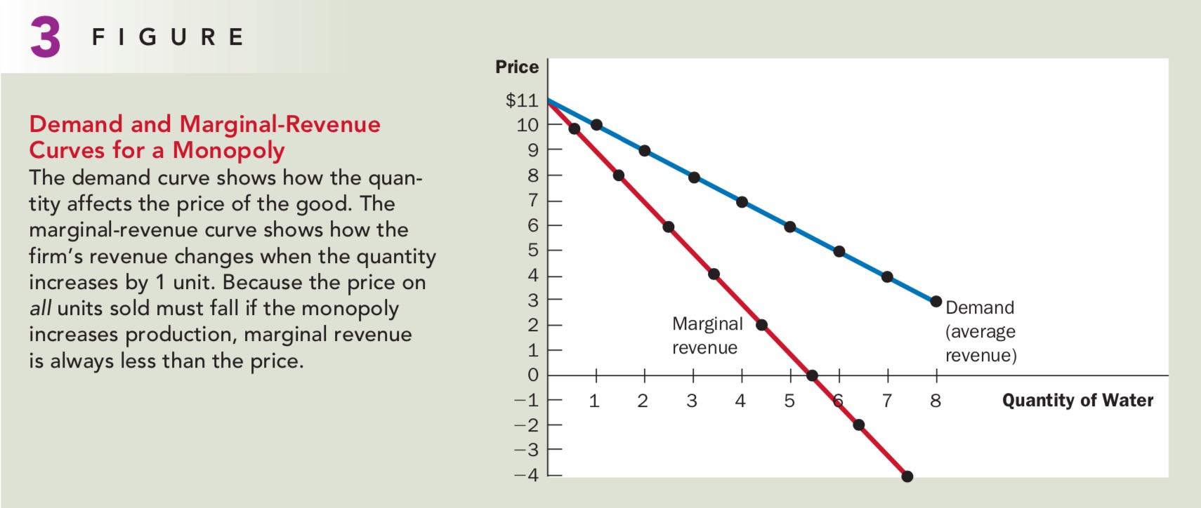
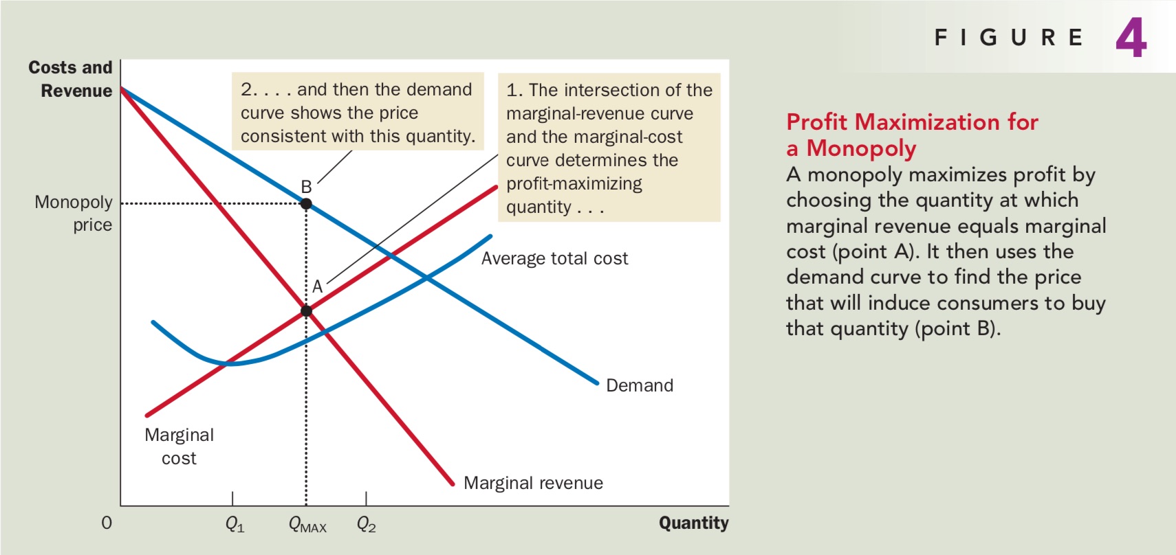
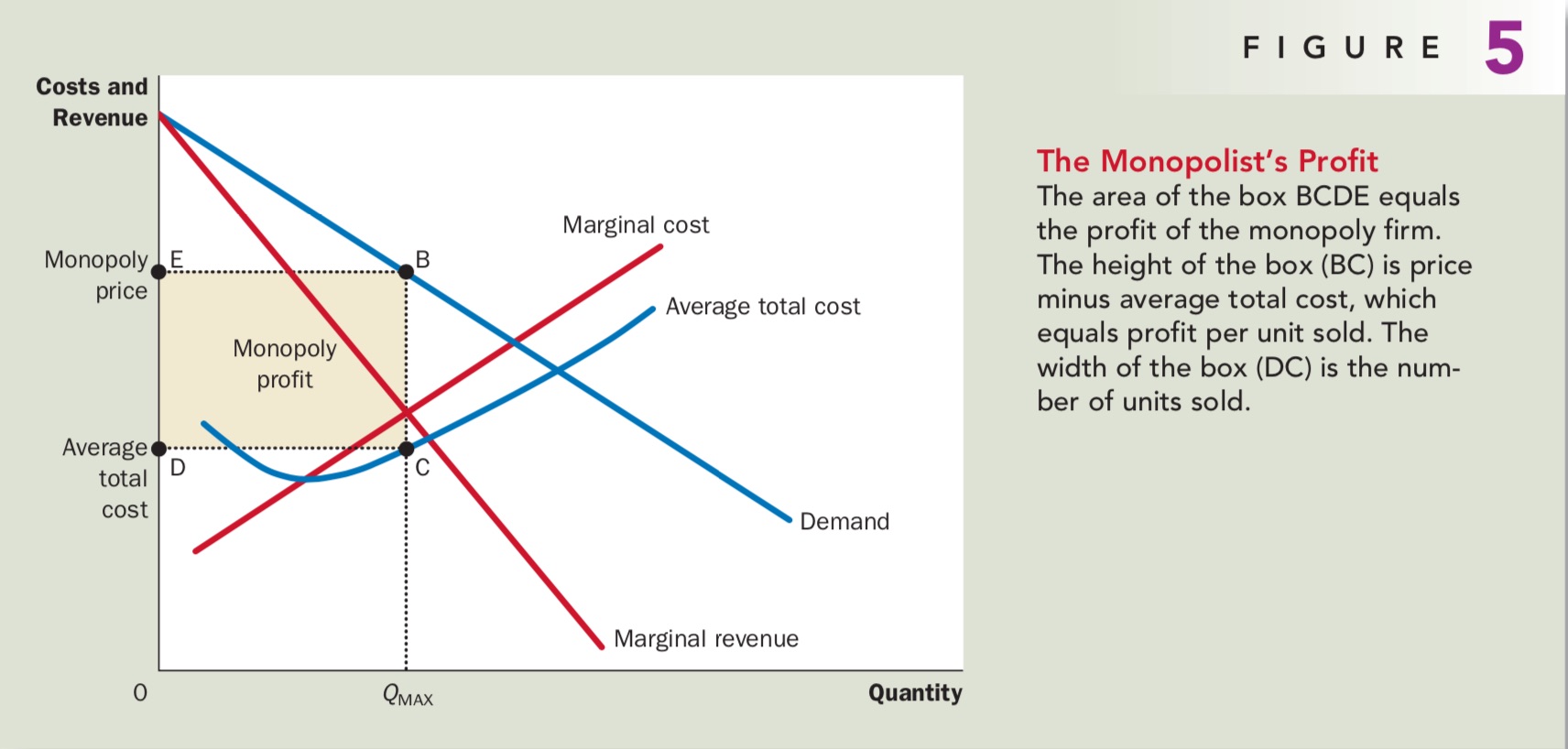
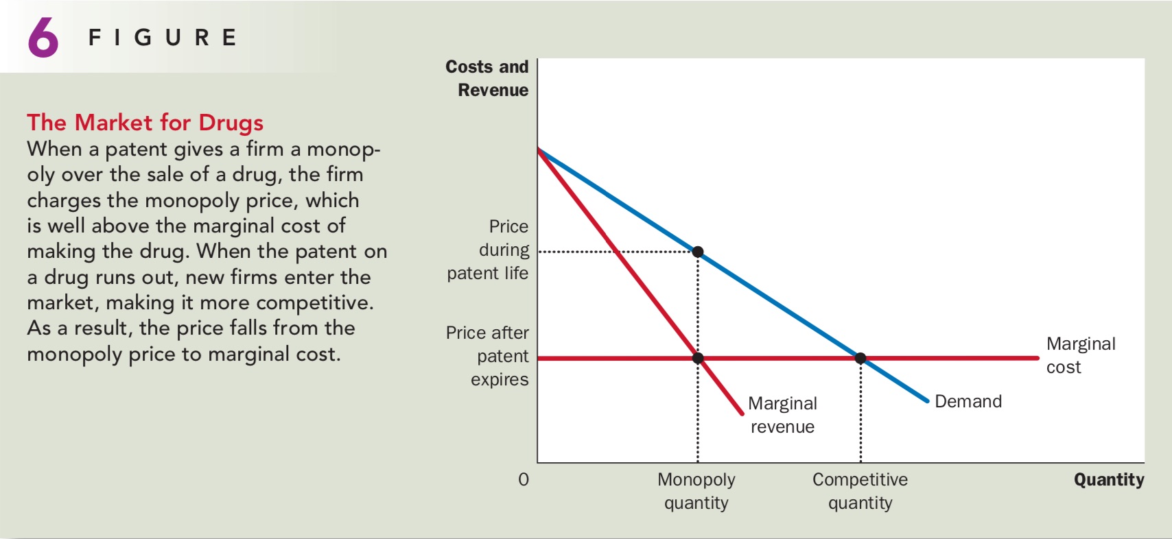
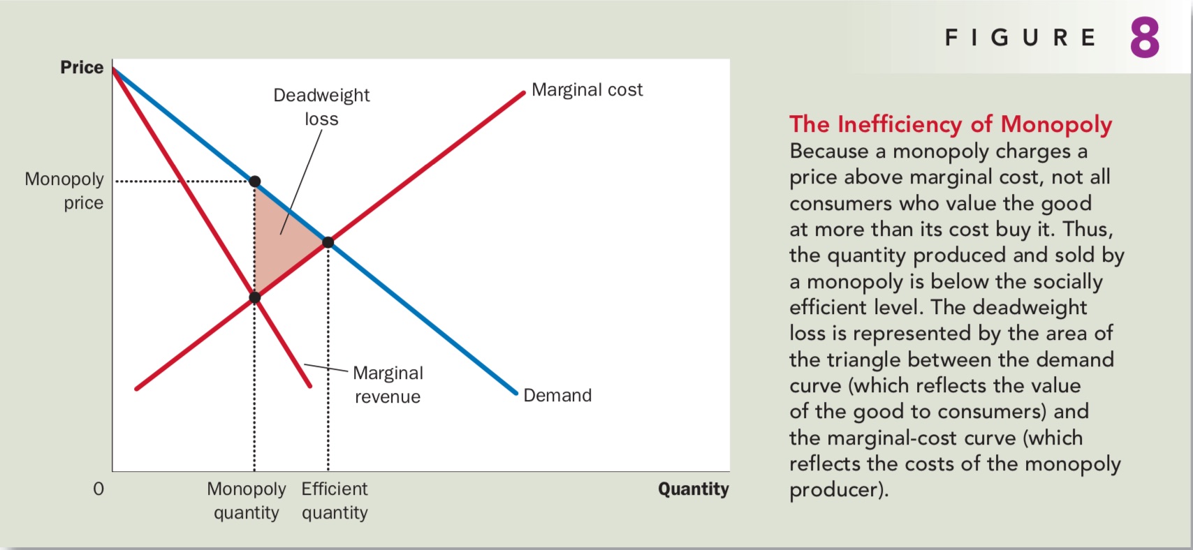
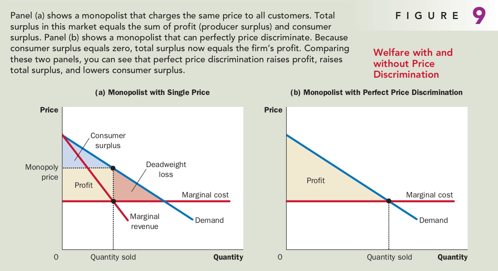
Monopoly - 完全垄断市场
完全垄断市场的特点(在没有价格歧视的情况下)
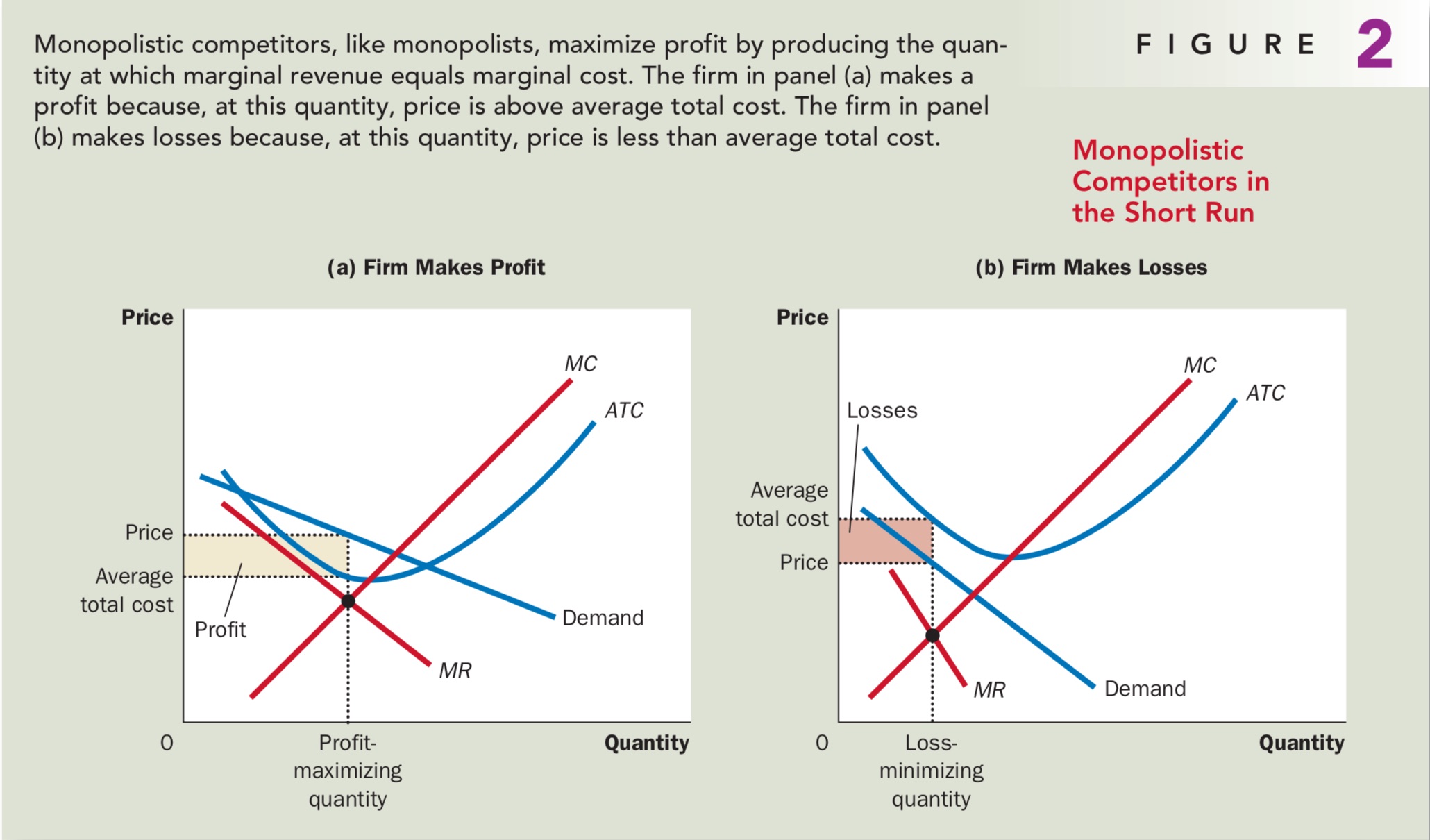
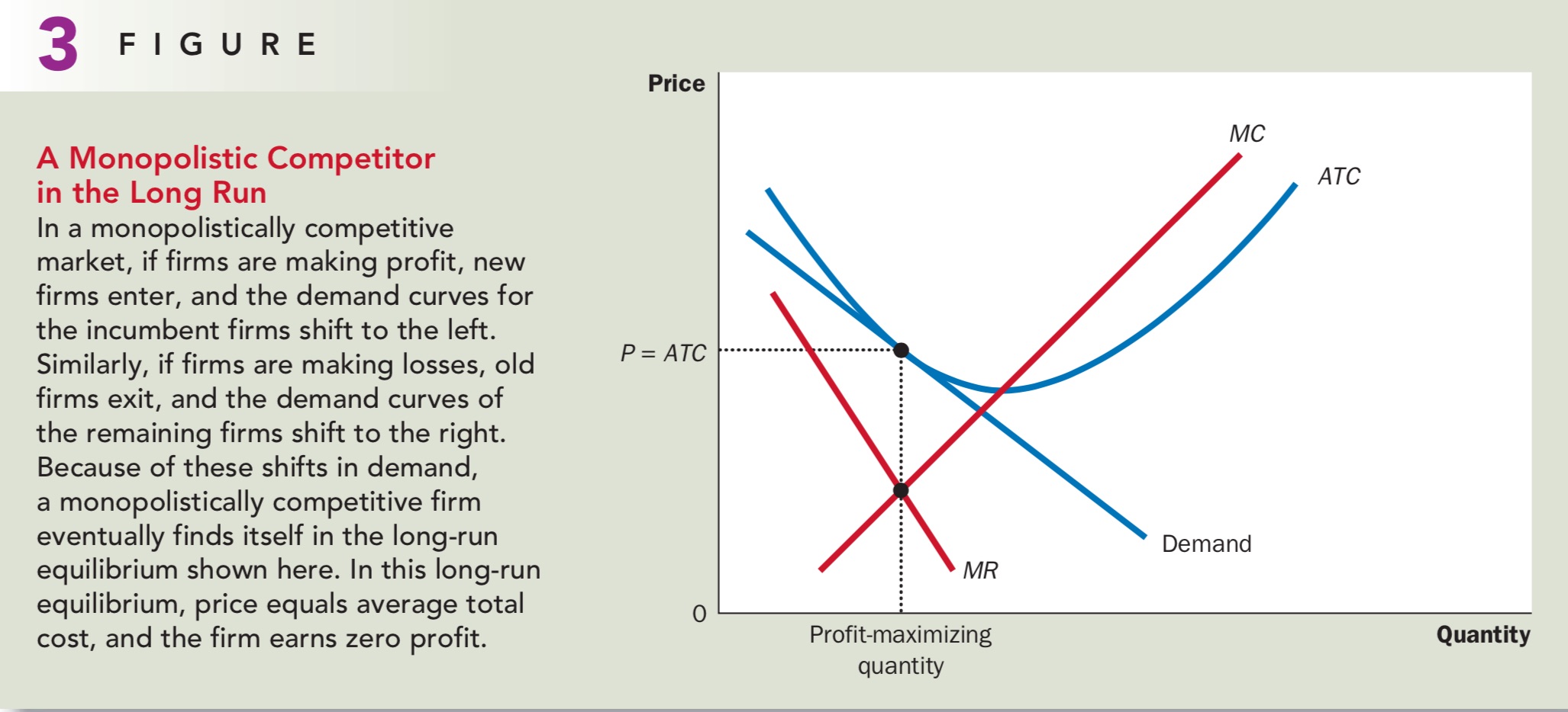
Monopolistic Competition - 垄断竞争
垄断竞争的特点
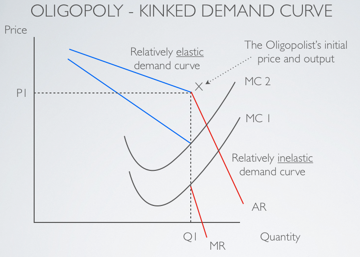
Oligopoly - 寡头垄断
就是几家企业搞垄断
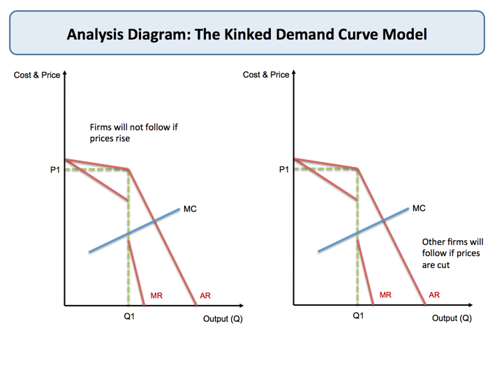
Kinked Demand Curve

生产要素市场 - The Markets for the Factors of Production
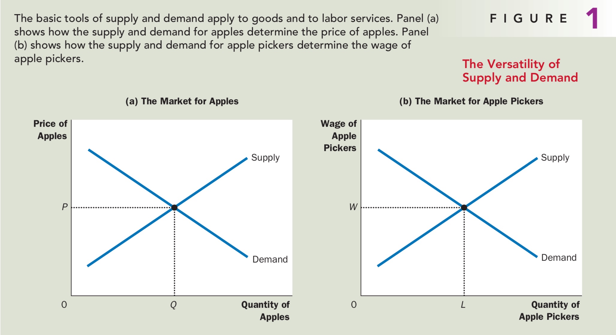
劳动的需求和供给的图像
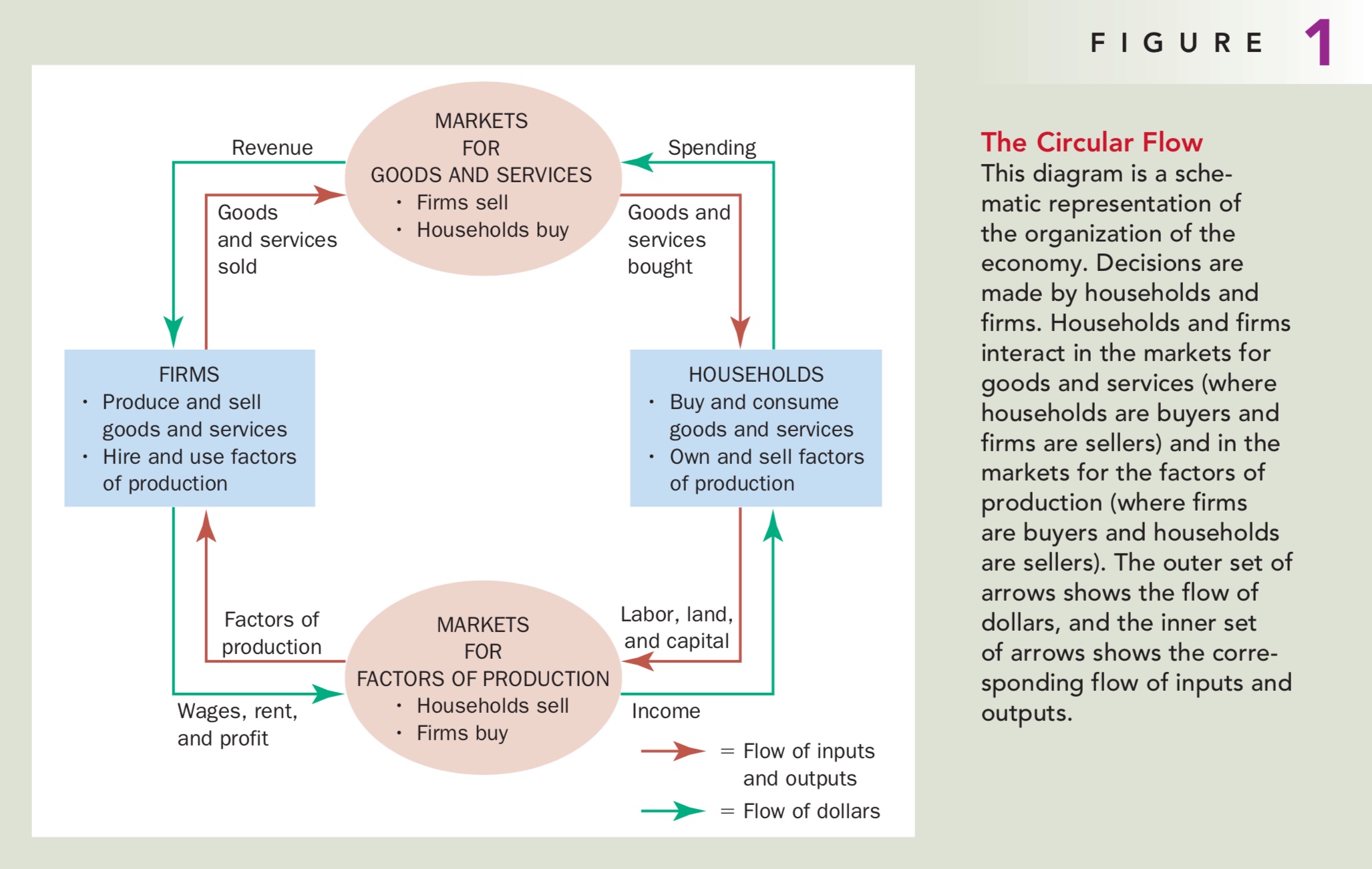
根据前面提到的循环流向图(Circular Flow Diagram),在生产要素市场当中企业是生产要素的购买者,家庭是生产要素的提供者。图像与之前商品市场中的图像基本相同(包括图像变动),不同之处在于纵轴从价格$P$变为了工资$\text{Wages}(W)$,横轴还是$\text{Quantity}(Q)$(只不过是Labour的数量)
在生产要素市场中Profit Maximizing
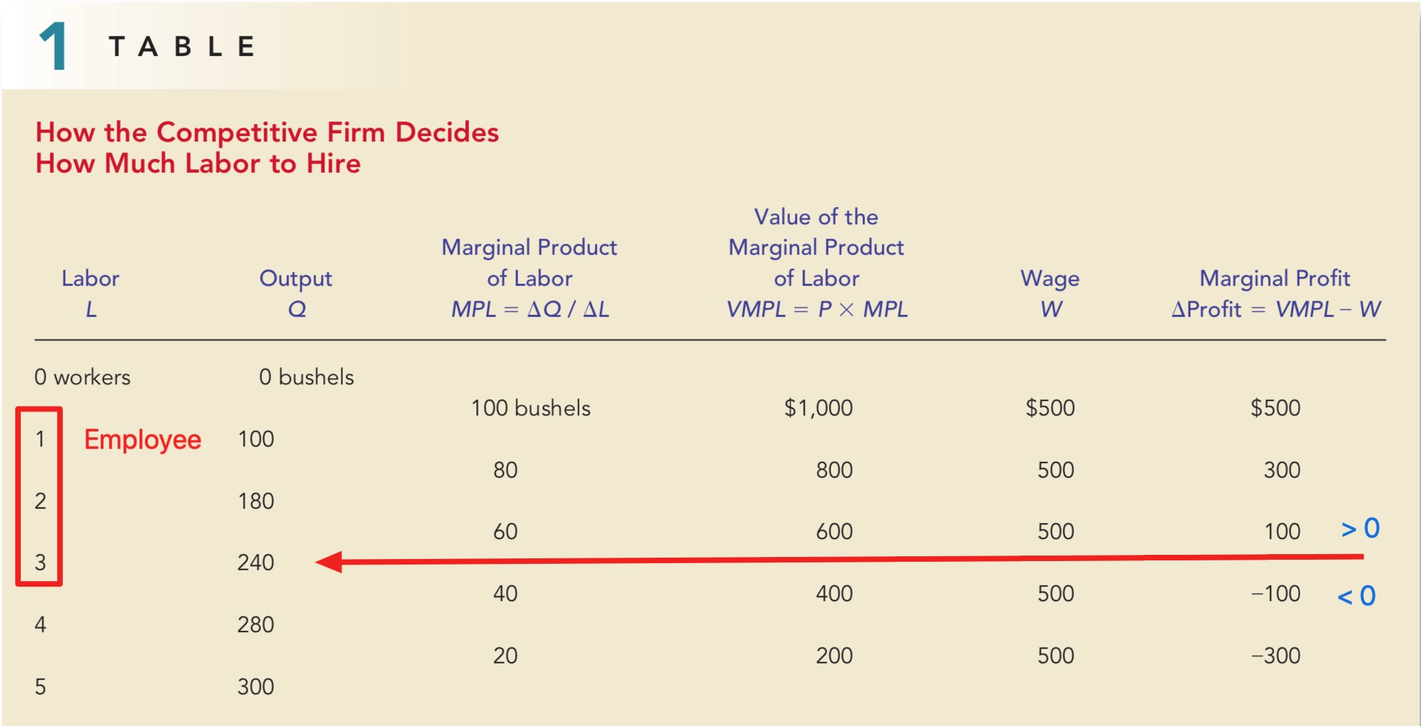
根据边际产量递减性质:$\text {Marginal Product of Labour} (MP_L)$是递减的,而每多雇佣一名工人能给企业带来的利润:$\text {Value of the Marginal Product of Labour}(VMPL)$,又称$\text {Marginal Revenue of Product (of Labour)} (MRP_L)$为:$P \times MP_L$。不难理解,只有当工人带来的收益大于成本才会雇佣,即$MRP_L > \text {Wages}$。
例如下表:
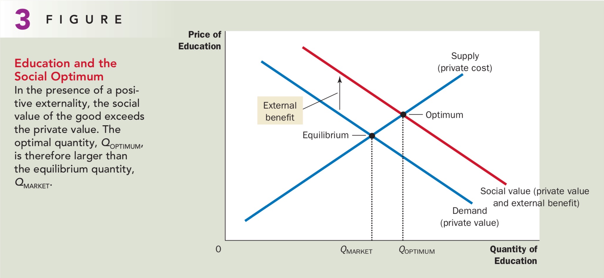
Externality - 外部性
- Positive Externality: 做一件事对别人有好处
- Negative Externality: 做一件事对别人有坏处
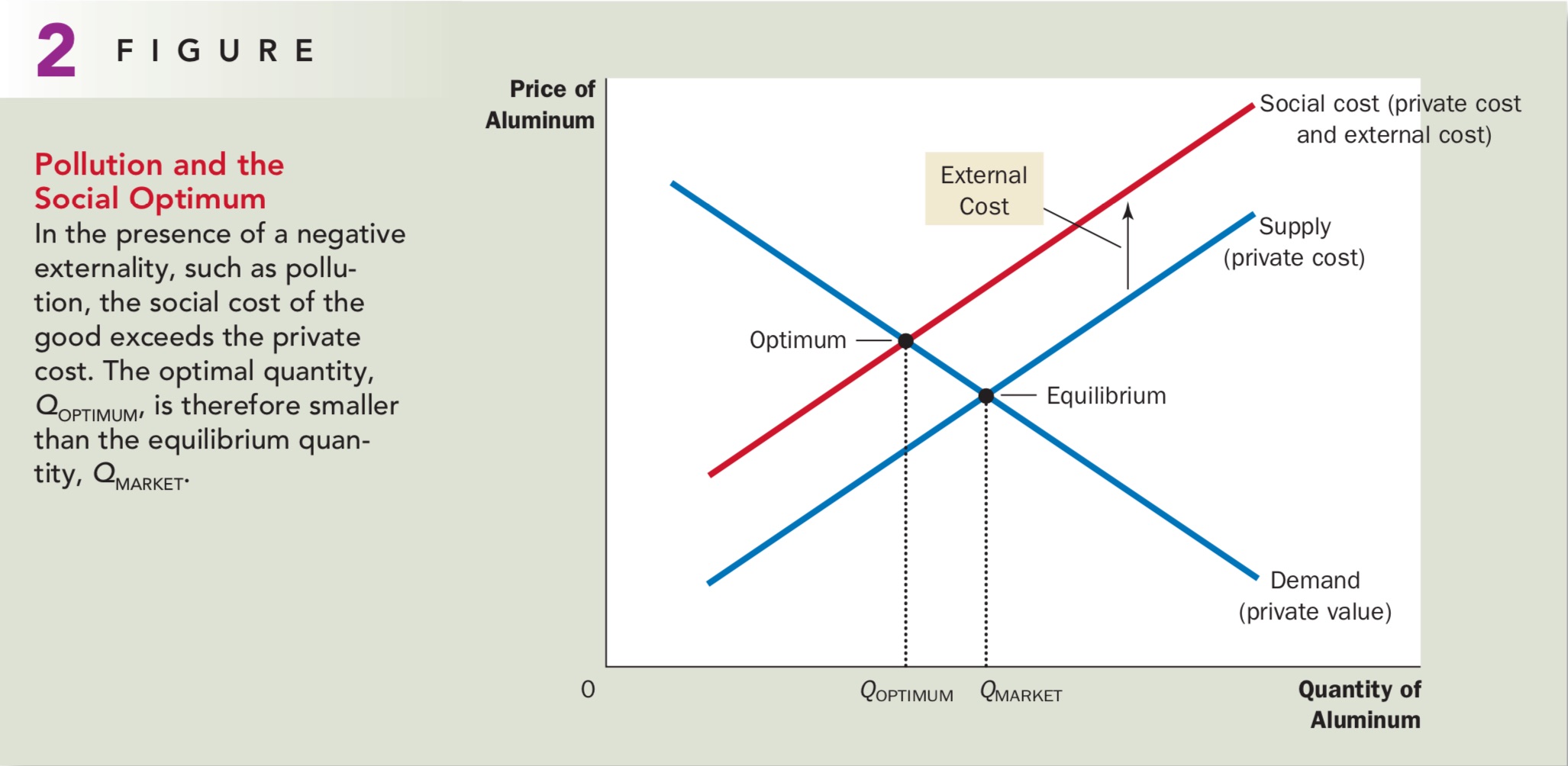
Negative Externality - 负外部性
负外部性的曲线
理解:因为做一件事对别人有不好的影响,所以供给曲线如果算上社会付出的成本的话,供给曲线需要上移,但是整个需求是没有变化的。
注:注意Social Optima和Market Equilibrium
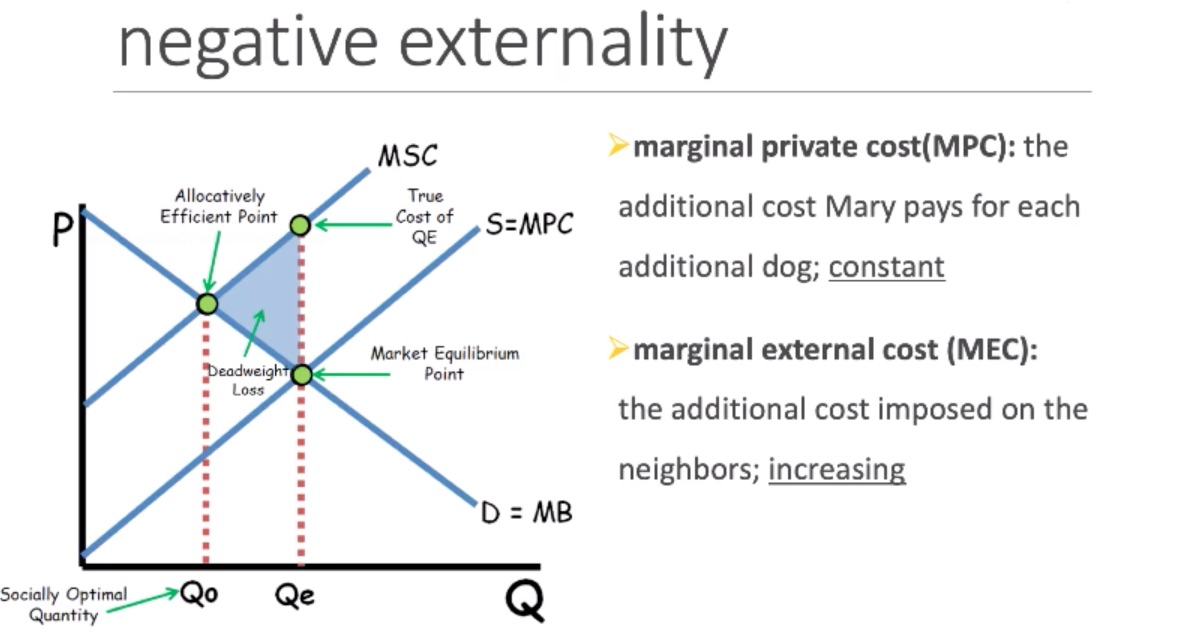
负外部性的最优实现
外部性内在化(Internalizing the Externality :对生产者进行收税,让生产者考虑自己的行为。

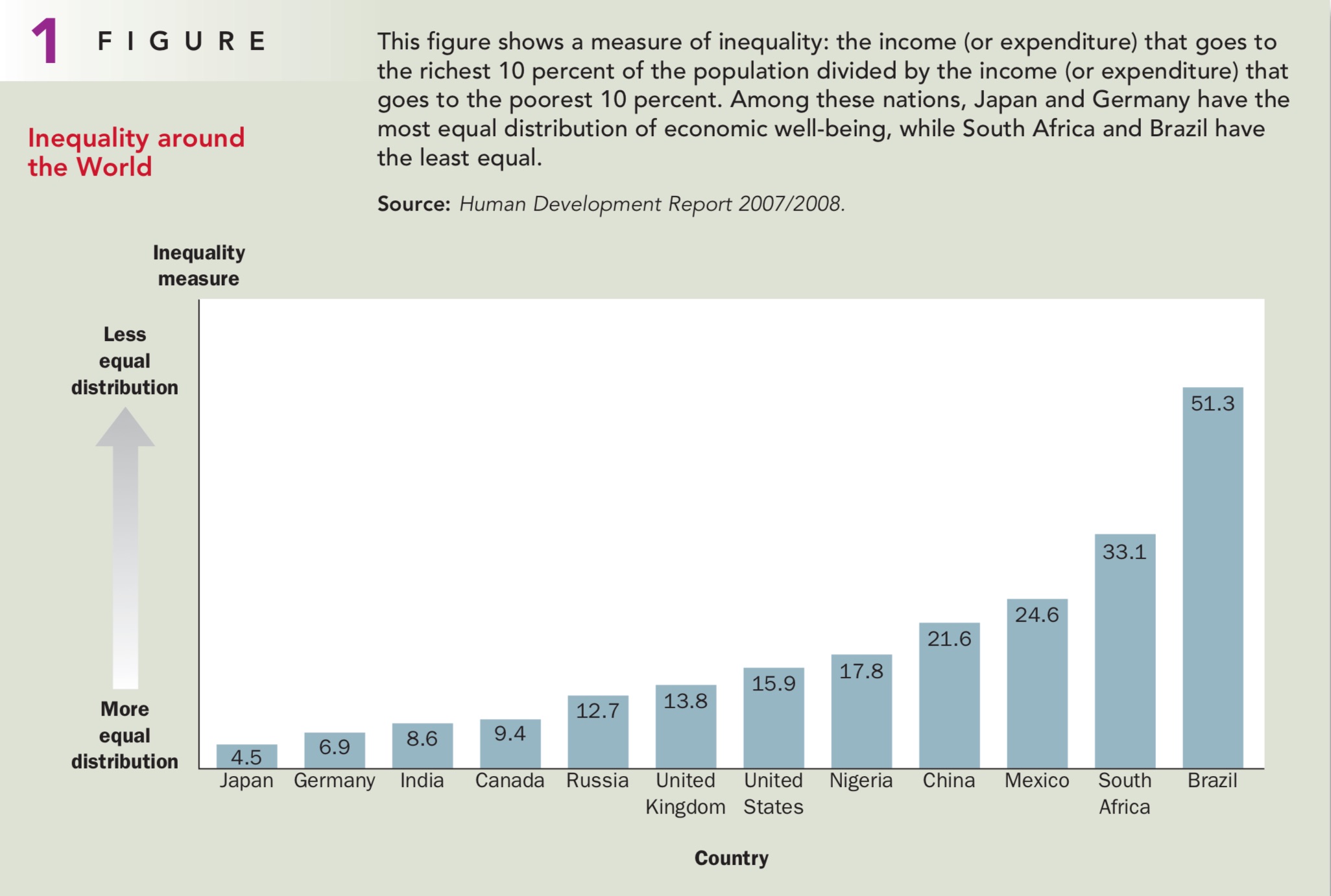
收入不平等
世界的收入不平等
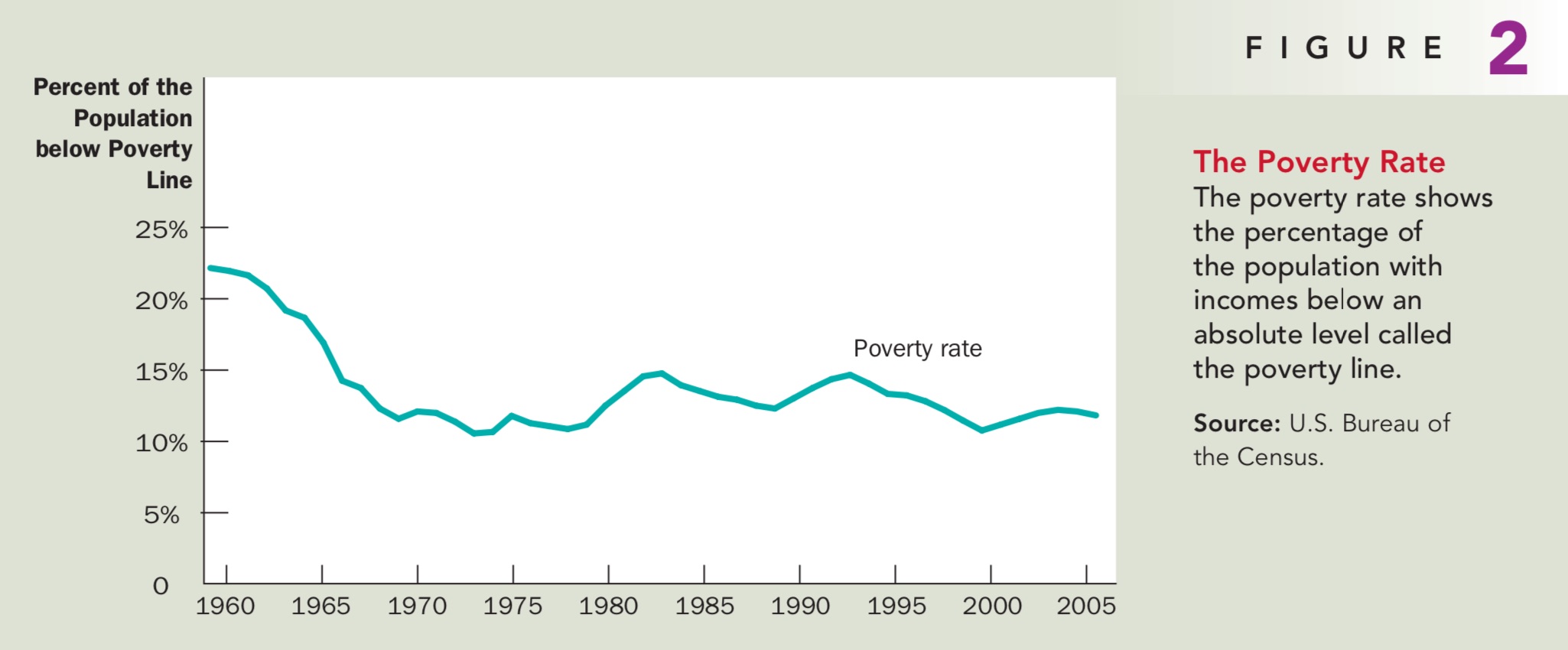
穷困率 - Poverty Rate
- 穷困率:家庭收入低于穷困线的人百分比
- 穷困线:政府制定的标准,低于这个水平就属于生活在贫困之中
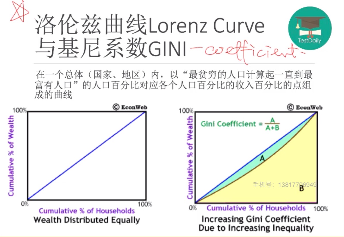
洛伦兹曲线和基尼系数 Lorenz Curve & Gini Coefficient
在一个总体(国家、地区)内,以“最贫穷的人口计算起一直到最富有人口”的人口百分比的收入百分比的点组成的曲线。
- 曲线越靠里,越极端,收入越不平等
- 曲线越接近 y = x(基准线),收入越平等
胜利在望!!最后一章!
消费者选择理论
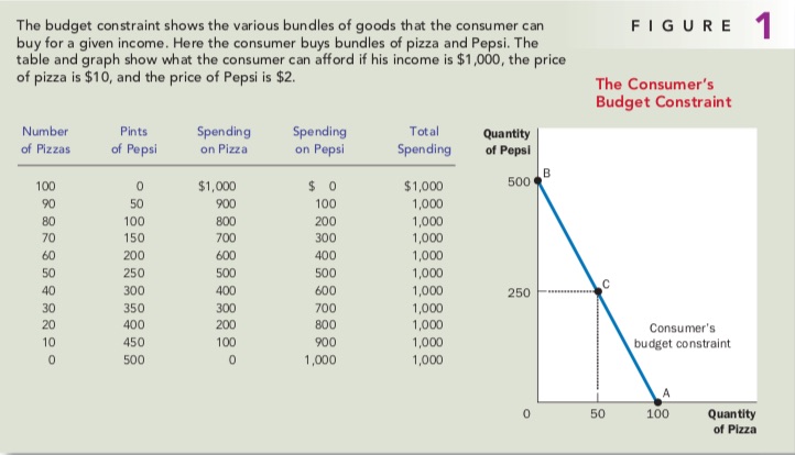
预算约束 - Budget Constraint
人话:因为只有这么点钱,所以会有限制和约束
无差异曲线 - Indifference Curve
又称Utility Curve。四个性质:
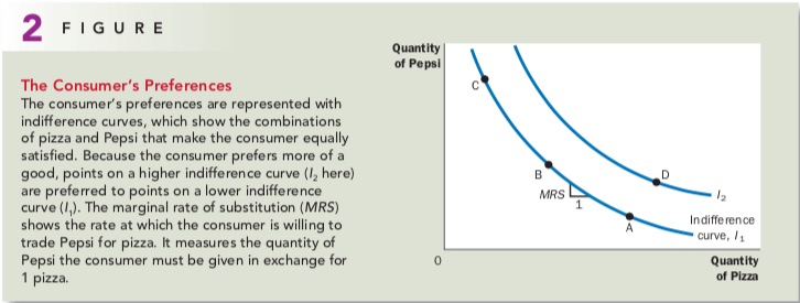
• Property 1: Higher indifference curves are preferred to lower ones. People usually prefer to consume more goods rather than less. This preference for greater quantities is reflected in the indifference curves. As Figure 2 shows, higher indifference curves represent larger quantities of goods than lower indiffer- ence curves. Thus, the consumer prefers being on higher indifference curves.
• Property 2: Indifference curves are downward sloping. The slope of an indiffer- ence curve reflects the rate at which the consumer is willing to substitute one good for the other. In most cases, the consumer likes both goods. Therefore, if the quantity of one good is reduced, the quantity of the other good must increase for the consumer to be equally happy. For this reason, most indiffer- ence curves slope downward.
• Property 3: Indifference curves do not cross. To see why this is true, suppose that two indifference curves did cross, as in Figure 3. Then, because point A is on the same indifference curve as point B, the two points would make the consumer equally happy. In addition, because point B is on the same indif- ference curve as point C, these two points would make the consumer equallyhappy. But these conclusions imply that points A and C would also make the consumer equally happy, even though point C has more of both goods. This contradicts our assumption that the consumer always prefers more of both goods to less. Thus, indifference curves cannot cross.
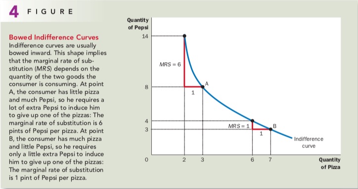
• Property 4: Indifference curves are bowed inward. The slope of an indifference curve is the marginal rate of substitution—the rate at which the consumer is willing to trade off one good for the other. The marginal rate of substitu- tion (MRS) usually depends on the amount of each good the consumer is currently consuming. In particular, because people are more willing to trade away goods that they have in abundance and less willing to trade away goods of which they have little, the indifference curves are bowed inward. As an example, consider Figure 4. At point A, because the consumer has a lot of Pepsi and only a little pizza, he is very hungry but not very thirsty. To induce the consumer to give up 1 pizza, he has to be given 6 pints of Pepsi: The marginal rate of substitution is 6 pints per pizza. By contrast, at point B, the consumer has little Pepsi and a lot of pizza, so he is very thirsty but not very hungry. At this point, he would be willing to give up 1 pizza to get 1 pint of Pepsi: The marginal rate of substitution is 1 pint per pizza. Thus, the bowed shape of the indifference curve reflects the consumer’s greater willingness to give up a good that he already has in large quantity.
注:不同的IC充满了整个平面
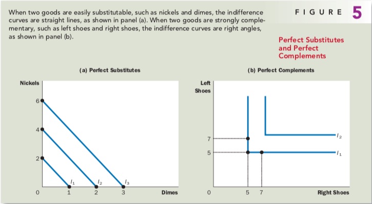
极端的IC曲线
消费者的选择
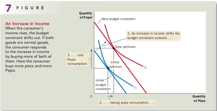
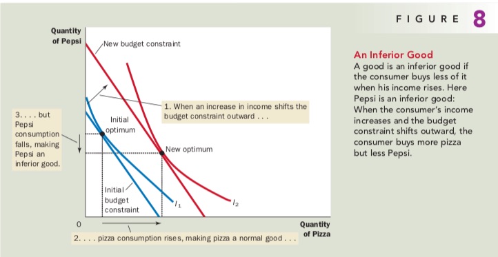
收入的变动 与 Normal Good 和 Inferior Good
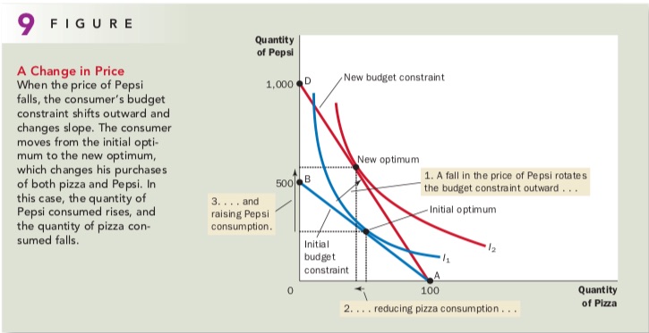
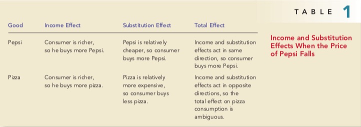
价格的变动 与 Substitution Effect 和 Income Effect
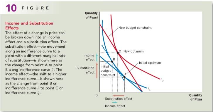
吉芬商品 - Giffen Good
价格增加,需求升高的商品
Utility - 效用
- 可以理解为benefit。
- 边际效用 - Marginal Utility
- 重点: Diminishing Marginal Utility:消费者拥有某商品越多,在额外增加一单位,带来的快乐低。
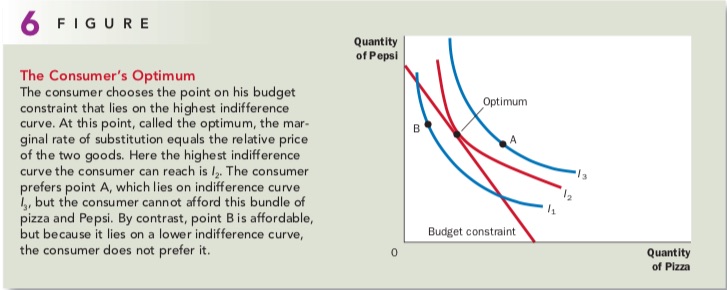
Optimal Consumption Bundle(重要)
其中,$P$为单价。
AP 2020 特辑
考试信息
- 考试时间:北京时间5月21日凌晨4点
- 两道FRQ
- Question 1 (55%): 25 minutes + 5 minutes to upload response
- Question 2
- 删减一个单元
Unit 6 Market Failure and the role of Government (8% - 13%) - Q1 = FRQ2 + FRQ3
- Q2 = FRQ1
考点
| Units | Exam Weighting |
|---|---|
| Unit 1: Basic Economic Concepts | 12-15% |
| Unit 2: Supply and Demand | 20-25% |
| Unit 3: Production, Cost, and the Perfect Competition model | 22-25% |
| Unit 4: Imperfect Competition | 15-22% |
| Unit 5: Factor Markets | 10-13% |
考察重点
- Unit1需要明确 definition
- Unit2几乎一定会融合在不同市场形式中考察(Unt3+4+5)
- 从完全竞争(side- by-side graph)/完全垄断/垄断竞争市场的图像中考察需求、供给曲线,弹性等
- Unit3-4一定会出1道题
- 市场之间的转化(垄断竞争完全竞争、寡头垄断-完全垄断)
- 每个市场的图像变化及结论
- Unit5有可能单独出题,其中一定会包含Unit2的知识点
Unit 1 - FRQ - 1
Nirali is a student at the University of Ainsley. She has 5 hours to study for two exams today. The tables below show Nirali’s expected scores given the amount of time she studies for each exam.
| Number of hours Spent Studying Microeconomics | Expected Score on Microeconomics exam (100-point scale) |
|---|---|
| 5 | 100 |
| 4 | 96 |
| 3 | 90 |
| 2 | 82 |
| 1 | 60 |
| 0 | 0 |
| Number of hours Spent Studying History | Expected Score on History exam (100-point scale) |
|---|---|
| 0 | 0 |
| 1 | 40 |
| 2 | 60 |
| 3 | 72 |
| 4 | 77 |
| 5 | 80 |
(a) Nirali spends 3 hours studying microeconomics and 2 hours studying history. Calculate her gain from the second hour spent studying history.
Solution: $40 \rightarrow 60$, $20$ points on History Exam.
(b) Calculate Nirali’s opportunity cost of the second hour spent studying history.
Solution: $6$ points on Microeconomics Exam.
(c) Assume Nirali increases the time she allocates to studying history. What happens to the opportunity cost of studying history? Explain
Solution: The opportunity cost of studying history will increase.
Explanation:
- Method 1: Expected score on Microeconmics decreases at an increasing rate for each hour spent on histroy.
- Method 2: Marginal cost is increasing.
(d) Assume that nirali has a goal of maximizing the sum of her test scores( the score on microeconomics plus the score on history). How many hours should she study for each exam?
Solution: She should study Microeconomics for $2$ hours and study Histroy for $3$ hours, which will enable her to achieve a total score of $154$ points, the maximum total score she can get.
(e) Nirali learns that her tennis practice has been canceled, freeing up an additional hour for studying. Given your answer to part(d), will Nirali allocate the additional hour to studying microeconomics or to studying history to maximize the sum of her test scores? Explain using marginal analysis
Solution: She will allocate the additional hour to studying microeconomics.
Explanation: Because the marginal benefit of learning an additional hour of microeconomics is $90 - 82 = 8$ points and the marginal benefit of learning an additional hour of history is $77 - 72 = 5$. $8 > 5$.
Unit 1 - FRQ - 2
Sasha is a utility-maximizing consumer who spends all of her income on peanuts and bananas, both of which are normal goods
- (a) Assume that the last unit of peanuts consumed increased Sasha’s total utility from 40 utils to 48 utils and that the last unit of bananas consumed increased her total utility from 52 utils to 56 utils
- (i) If the price of a unit of peanuts is SI and Sasha is maximizing utility, calculate the price of a unit of bananas
- Solution: Thus the price of banana is $(56 - 52) \div (48 - 40) \times 1 = 0.5$ dollars
- (ii) If the price of a unit of peanuts increases and the price of a unit of bananas remains unchanged from the price you determined in part(a)(i), how will Sasha’s purchase of peanuts change?
- Solution: She will purchase less peanuts.
- (b) Assume that the cross-price elasticity of demand between peanuts and bananas is positive. A widespread disease has destroyed the banana crop. What will happen to the equilibrium price and quantity of peanuts in the short run? Explain
- (c) Assume that the price of bananas increases.
- (i) Will the substitution effect increase, decrease, or have no effect on the quantity of bananas demanded?
- (ii) What happens to Sasha’s real income?
Unit 2 - FRQ - 1
The graph below shows the market for widgets. The government is considering intervening in this market.
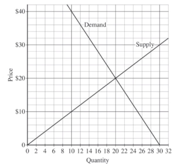
- (a) Calculate the total producer surplus at the market equilibrium price and quantity. Show your work.
- Solution: $20 \times 20 \div 2 = 200$ dollars
- (b) If the government imposes a price floor at $16, is there a shortage, a surplus, or neither? Explain
- Solution: Neither, because the price floor is below the equilibrium, thus it is not binding / not effective / ineffective.
- (c) If instead the government imposes a price ceiling at $12, is there a shortage, a surplus, or neither? Explain
- Solution: There will be a shortage, because the price ceiling is below the equilibrium and $Q_D > Q_S$ (Quantity Demanded is greater than Quantity Supplied).
- (d) If instead the government restricts the market output to 10 units, calculate the deadweight loss. Show your work.
- Solution: $(40 - 10) \times (20 - 10) \div 2 = 150$ dollars.
- (e) Assume the price decreases from 20 dollars to 12 dollars.
- (i) Calculate the price elasticity of demand. Show your work.
- Solution:
- (ii) In this price range, is demand perfectly elastic, relatively elastic, unit elastic, relatively inelastic, or perfectly inelastic?
- Solution: Since $\varepsilon < 1$, the demand is relatively inelastic in this price range.
Unit 2 - FRQ - 2
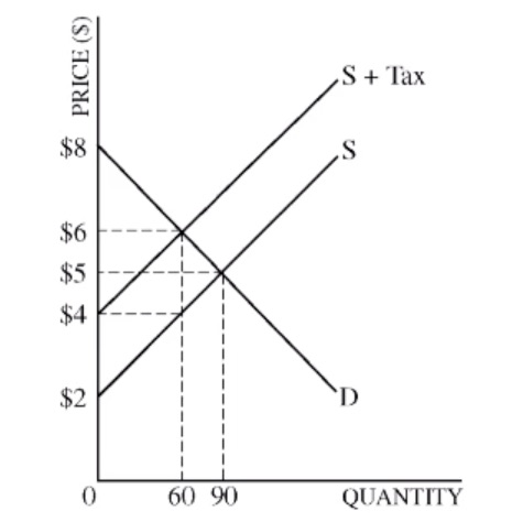
The graph above illustrates the market for calculators. S denotes the current supply curve, and D denotes the demand curve.
- (a) Calculate the producer surplus before the tax
- Solution: $(5 - 2) \times 90 \div 2 = 135$ dollars.
- (b) Now assume a per-unit tax of $2 is imposed whose impact is shown in the graph above.
- (i) Calculate the amount of tax revenue.
- Solution: $2 \times 60 = 120$ dollars.
- (ii) What is the after-tax price that the sellers now keep?
- Solution: $4$ dollars.
- (iii) Calculate the producer surplus after the tax.
- Solution: $(4 - 2) \times 60 \div 2 = 60$ dollars.
- (c) Is the demand price elastic, inelastic, or unit elastic between the prices of 5 dollars and 6 dollars? Explain.
- Solution:
- Method 1:Since $\varepsilon > 1$, the demand price is elastic between the prices of 5 dollars and 6 dollars.
- Method 2: When price change from $5$ dollars to $6$ dollars, the total revenue decreases, thus the price demand is elastic.
- (d) Assuming no externalities, how does the tax affect allocative efficiency? Explain
- Solution:
- Method 1: It produced deadweight loss.
- Method 2: The Consumer Surplus and Producer Surplus decreased.
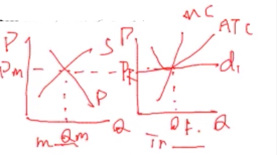
Unit 3 - FRQ - 1
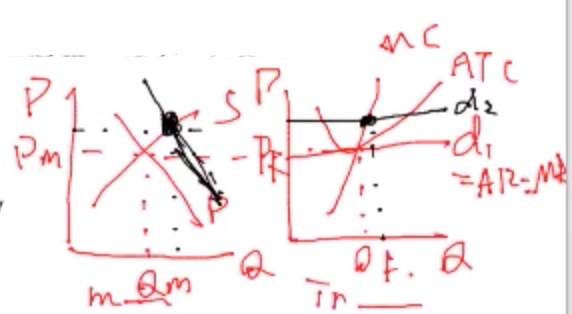
Suppose that roses are produced in a perfectly competitive, increasing-cost industry in long-run equilibrium with identical firms.
- (a) Draw correctly labeled side-by-side graphs for the rose industry and a typical firm and show each of the following
- (i) Industry equilibrium price and quantity, labeled $P_m$ and $Q_m$, respectively
- (ii) The firms equilibrium price and quantity, labeled $P_f$ and $Q_f$ respectively

- (b) Is $P_m$ larger than, smaller than, or equal to $P_f$?
- Solution: $P_m = P_f$
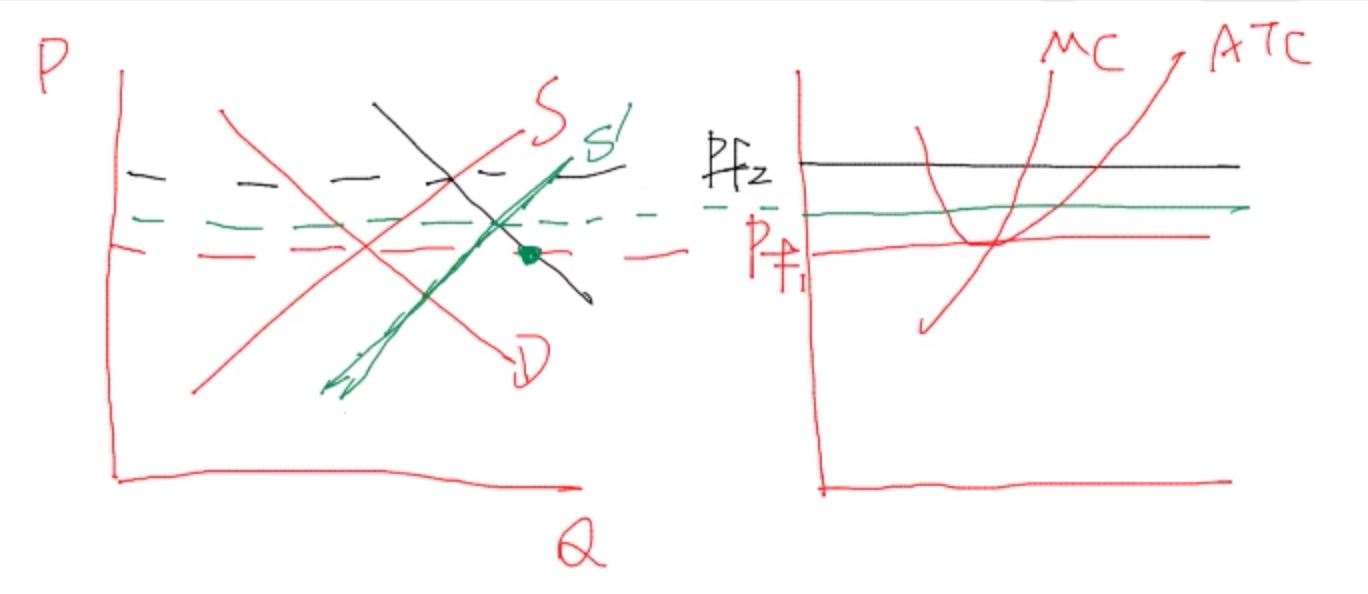
- (c) Assume that there is an increase in the demand for roses On your graphs in part(a), show each of the following.
- (i) The new short-run industry equilibrium price and quantity, labeled $P_{m2}$ and $Q_{m2}$, respectively
- (ii) The new short-run profit-maximizing price and quantity for the typical firm, labeled $P_{f2}$ and $Q_{f2}$, respectively
- (d) As the industry adjusts to a new long-run equilibrium,
- (i) what will happen to the number of firms in the industry? Explain
- Solution: The number of firms in the industry will increase. Since the profit $\pi = (P - ATC) \times Q > 0$, the existence profit attracts to enter the industry and there is no barrier of entering the market, there will be more firms in the industry.
- (ii) Will the firm’s average total cost curve shift upward, shift downward, or remain unchanged?
- Solution: It will shift upward for the reason that it is an Increasing-cost Industry.
- (e) In the long run, compare the firm’s profit-maximizing price to each of the following
- (i) $P_f$ in part(a)(ii)
- Solution: $P > P_f$, Higher
- (ii) $P_{f2}$ in part(c)(ii)
- Solution: $P < P_{f2}$, Lower
Unit 4 - FRQ - 1
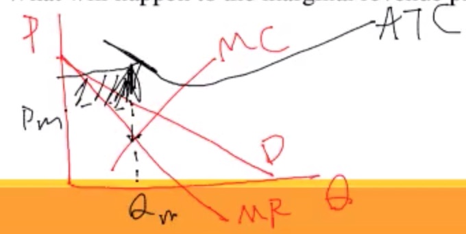
In the early twentieth century, limited transportation options and the lack of effective substitutes gave Single Cinema monopoly power in a small town. Assume that Single Cinema is a profit-maximizing firm and currently operates at a negative economic profit in the short run
- (a) Draw a correctly labeled graph for Single Cinema, and show each of the following
- (i) The profit-maximizing price and quantity of tickets, labeled as $P_m$ and $Q_m$, respectively
- (ii) The area representing the negative economic profit, shaded completely
- (b) Explain why Single Cinema continues to operate in the short run despite earning negative economic profit in the short run
- Solution: $P > AVC$
- (c)Would Single Cinema’s total revenue increase, decrease, or stay the same if it decides to sell one fewer ticket than $Q_m$? Explain.
- Solution:
- Method 1: $MR > 0$, $TR$ will decrease.
- Method 2: The demand curve is always elastic when $MR > 0$, thus total revenue will decrease when quantity decrease.
- (d) Single Cinema hires workers in a perfectly competitive labor market with a downward-sloping demand curve. Suppose the number of workers available in the market decreases
- (i) What will happen to the wage rate? Explain
- (ii) What will happen to the marginal revenue product of the last worker hired? Explain
Unit 4 - FRQ - 2
Mary Company, operating in a monopolistically competitive industry, produces a cleaning product called BriteKlean. The company currently produces the profit-maximizing quantity of BriteKlean but is operating at a loss.
- (a) Draw a correctly labeled graph for Mary Company and show each of the following
- (i) The profit-maximizing output and price, labeled as Q and PM, respectively
- (ii) The area of loss, shaded completely
- (b) what must be true in the short run for the company to continue to produce at a loss?
- (c) Assume now that the demand for cleaning products increases and that the company is now earning short-run economic profits. Relative to this short-run situation, how does each of the following change in the long run?
- (i) The number of firms
- (ii) The company’s profit
- (d) In the long run, if the company continues to produce, will it produce the allocatively efficient level of output? Explain
- (e)In the long run, will the company be operating in a region where economies of scale exist? Explain.
- Solution: It will operate in a region where economies of scale exist, because the firm is in a monopolistically competitive industry. In the long run, $P = ATC > \min ATC$, the firm will always produce where the slope of $ATC$ is negative, from which the company is operating in a region where economies of scale exist.
Unit 4 - FRQ - 3
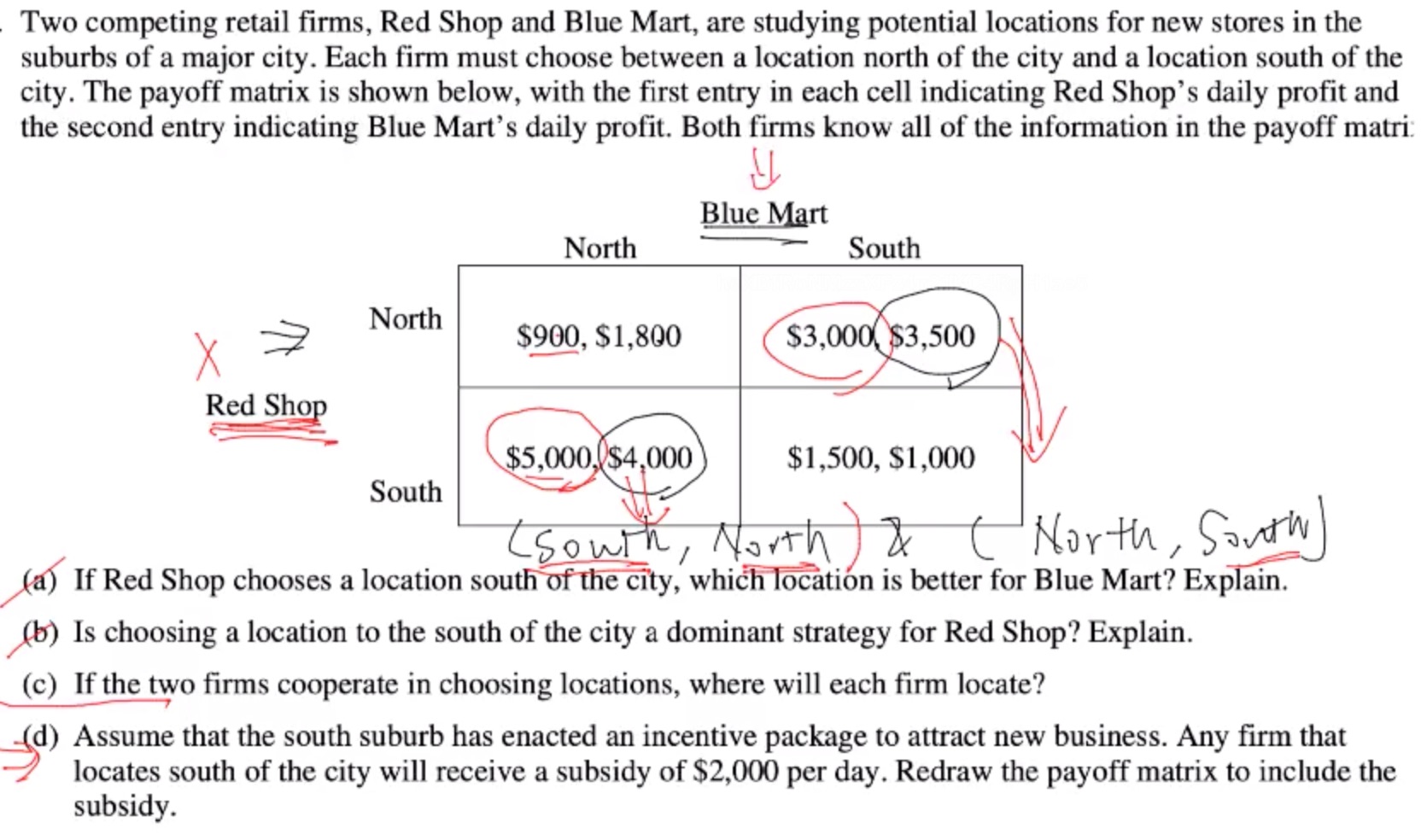
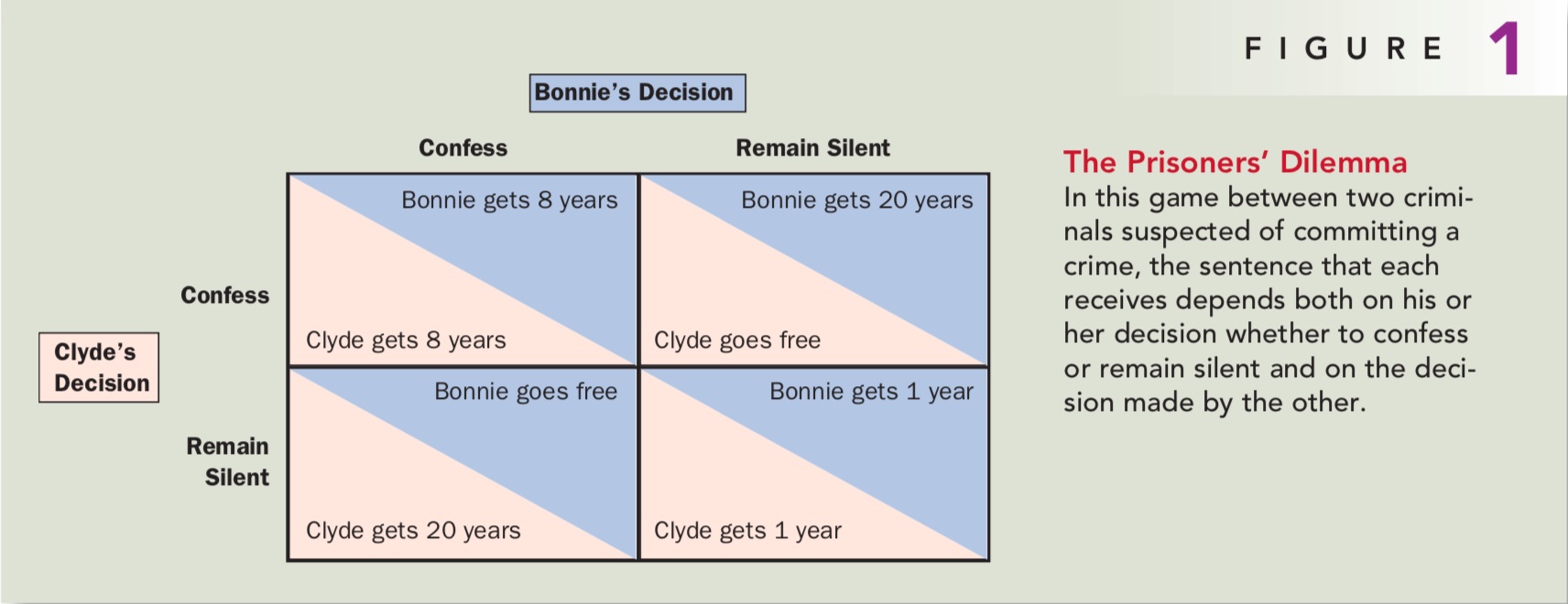
这一题当中,Nash Equilibrium有两个,已经在图片上标注出来了。做法:画圈圈出对手在不同情况下选择做出的Dominant Strategy或者Strategy,如果一个格子里有两个公司的圈就是均衡。
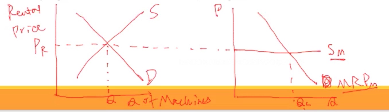
Unit 5 - FRQ - 1
The John Lamb Company, a profit-maximizing firm producing widgets, is in a perfectly competitive widget market. Assume John Lamb employs a fixed number of employees and rents a machine for a variable number of hours from a perfectly competitive market
- (a) Using correctly labeled side-by-side graphs of the factor market for machines and the John Lamb Company, show each of the following
- (i) The equilibrium rental price of machines in the factor market, labeled as $P_R$
- (ii) John Lamb’s equilibrium rental quantity of machines, labeled as $Q_L$
- (b) Assume that the popularity of widgets declines, decreasing the demand for widgets. What will happen to each of the following?
- (i) Marginal product curve for machine-hours
- Solution: It will remain the same. $MP_M$ doesn’t relate with $P$
- (ii) Marginal revenue product curve for machine-hours. Explain.
- Solution: It will decrease, since $MR = P \times MP_M$, with $P$ decreasing, $MR$ will decrease too.
- (c) John Lamb is employing the cost-minimizing combination of inputs. The marginal product of labor is 28 widgets per worker hour and the wage rate is $14 per hour. The marginal product of the machine is 60 widgets per machine-hour. What is the hourly rental price of a machine?
Unit 5 - FRQ - 2 - Monopsony(单一Employer)
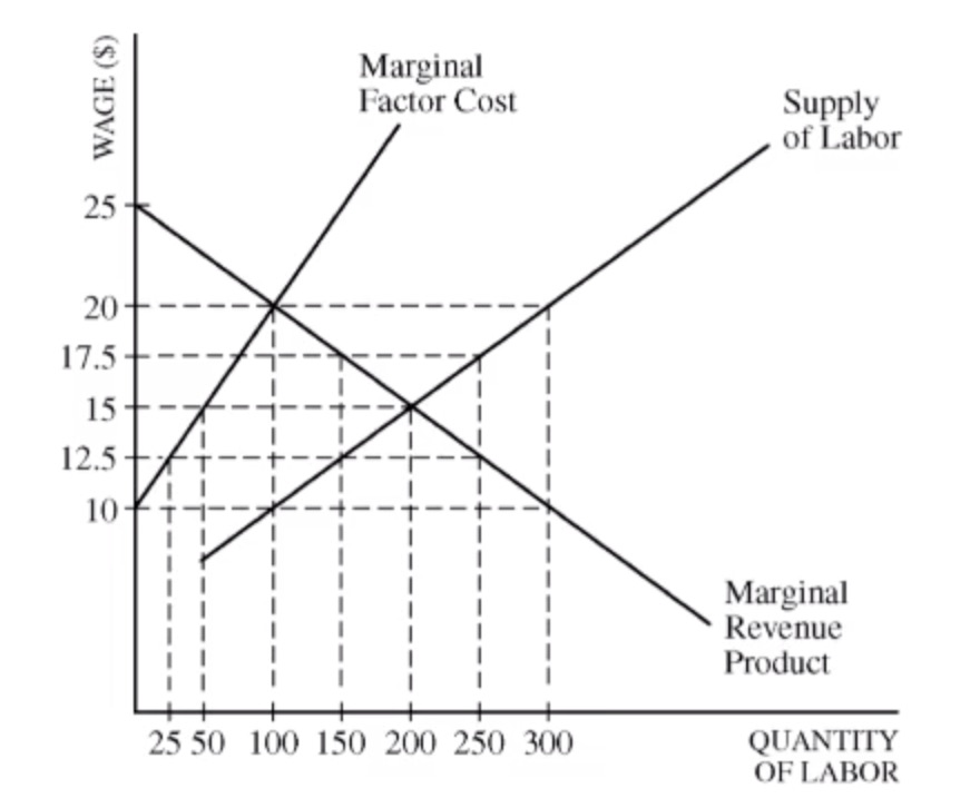
Woodland is a small town in which everyone works for TreeMart, the local lumber company. TreeMart is a monopsonist in the labor market and a perfect competitor in the lumber market. In the short run, labor is the only variable input. The labor market for TreeMart is given in the graph above
- (a) Identify the profit-maximizing quantity of labor for TreeMart
- Solution: $MC = MR$, 100.
- (b)Identify the wage rate Tree Mart pays to hire the profit-maximizing quantity of labor
- Solution: $10
- (c) Identify the quantity of labor hired in each of the following situations.
- (i) Tree Mart operates in a competitive labor market
- Solution: Competitive $\rightarrow S = D$, 200.
- (ii) The government imposes a minimum wage of $12.5 Explain.
- Solution: With the minimum wage of $12.5, according to the supply curve of labor, the company will hire 150 units of labor.
重要注意点
- 写清楚单位